天文数据处理 期末考试报告
姓名:韦境量
学号:202311160016
题目
读取数据
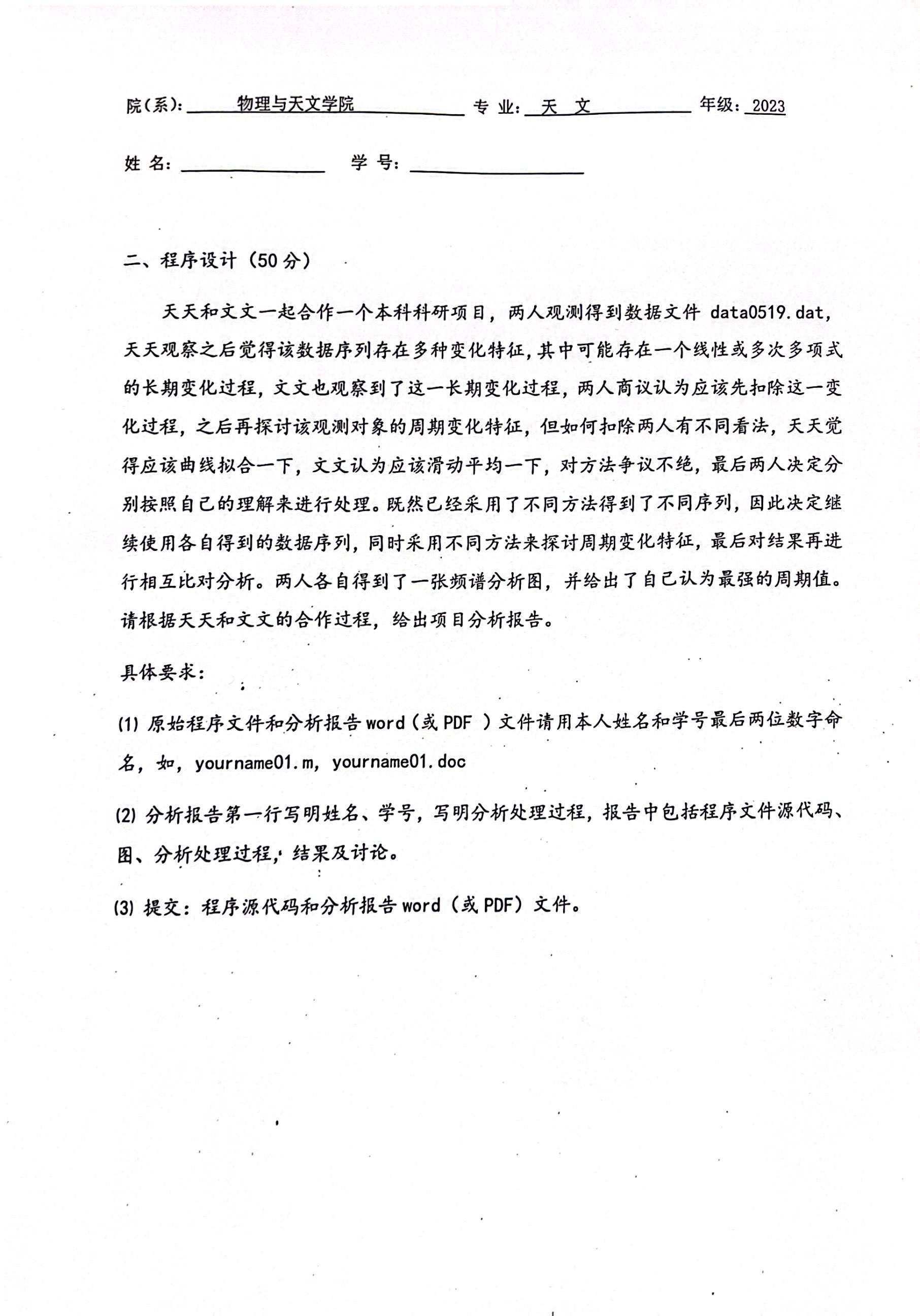
先读取数据并绘图观察,读取时去除表头和缺少值 NaN,编写 read.py:
py
import numpy as np
import matplotlib.pyplot as plt

# read time and data from file
time, data = [], []
file = open('data0519.dat', 'r')
istitle = True
for line in file:
    line = line.split()
    if istitle:
        istitle = False
        continue
    if line[3] == 'NaN':
        continue
    time.append(float(line[2]))
    data.append(float(line[3]))
file.close()
time = np.array(time)
data = np.array(data)

# draw the data-time
plt.plot(time, data)
plt.xlabel('time/yr')
plt.ylabel('data')
plt.show()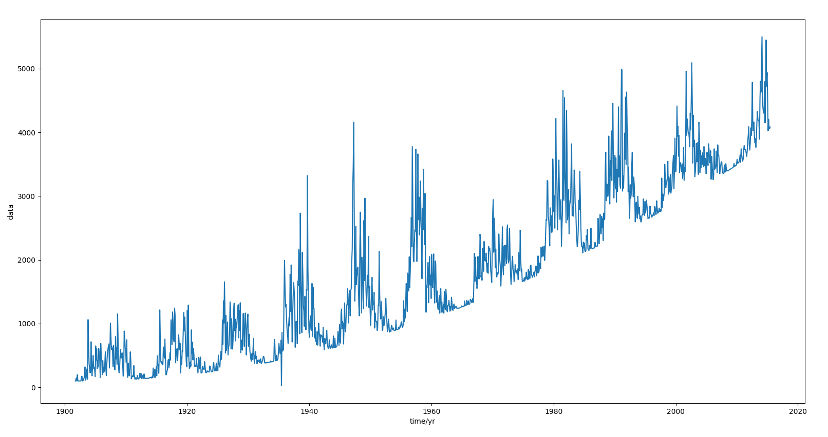
可以看到数据有一个二次多项式增长的趋势。
天天的处理
通过曲线拟合扣除趋势项,然后使用傅里叶变换进行频谱分析。
tt.py 代码逻辑
- 读取原始数据
time,data - 选取部分数据(每100个)进行二次多项式拟合得到多项式函数
f - 对原数据
data进行线性插值,转成时间间隔固定的时间序列(并且扣除趋势项f)得到time_uniform,data_uniform - 进行傅里叶变换 FFT 得到
fre,fft_abs - 绘图(原始数据和拟合曲线、预处理过的数据、傅里叶频谱图)
py
import numpy as np
import matplotlib.pyplot as plt
from scipy.interpolate import interp1d
from scipy.fftpack import fft

# read time and data from file
time, data = [], []
file = open('data0519.dat', 'r')
istitle = True
for line in file:
    line = line.split()
    if istitle:
        istitle = False
        continue
    if line[3] == 'NaN':
        continue
    time.append(float(line[2]))
    data.append(float(line[3]))
file.close()
time = np.array(time)
data = np.array(data)

# curve fit
time_fit = time[0:-1:100]
data_fit = data[0:-1:100]
an = np.polyfit(time_fit, data_fit, 2)
f = np.poly1d(an)

# remove trend and keep delta-t fixed by interpolate
time_uniform = np.linspace(time[0], time[-1], len(time))
data_interp = interp1d(time, data, kind='linear')
data_uniform = data_interp(time_uniform) - f(time_uniform)

# fft
N = len(time_uniform)
T = time_uniform[-1] - time_uniform[0]
fft_y = 2 * fft(data_uniform) / N
fft_abs = np.abs(fft_y)
fre = np.arange(N) / T

# draw the data-time
ax1 = plt.subplot(311)
ax2 = plt.subplot(312)
ax3 = plt.subplot(313)
ax1.plot(time, data, label='raw data')
ax1.plot(time, f(time), label='fit curve')
ax1.set_xlabel('time/yr')
ax1.set_ylabel('data')
ax1.legend()
ax2.plot(time_uniform, data_uniform, label='data after preprocessing')
ax2.set_xlabel('time/yr')
ax2.set_ylabel('data')
ax2.legend()
ax3.plot(fre, fft_abs, label='FFT')
ax3.set_xlabel(r'$f/yr^{-1}$')
ax3.set_ylabel('Magnitude')
ax3.legend()
plt.show()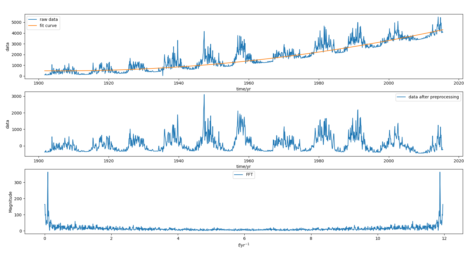
从频谱图中可以得到,最强的周期项频率为
文文的处理
通过滑动平均扣除趋势项,然后使用周期图法进行频谱分析。
ww.py 代码逻辑
- 读取原始数据
time,data - 进行窗长度为200的滑动平均
data_movavg - 对原数据
data和滑动平均数据data_movavg进行线性插值,转成时间间隔固定的时间序列(扣除趋势项data_movavg)得到time_uniform,data_uniform - 使用周期图法(periodogram)进行功率谱估计得到
fre,Pxx - 绘图(原始数据和滑动平均数据、预处理过的数据、功率谱图)
py
import numpy as np
import matplotlib.pyplot as plt
from scipy.signal import savgol_filter
from scipy.interpolate import interp1d
from scipy.signal import periodogram

# read time and data from file
time, data = [], []
file = open('data0519.dat', 'r')
istitle = True
for line in file:
    line = line.split()
    if istitle:
        istitle = False
        continue
    if line[3] == 'NaN':
        continue
    time.append(float(line[2]))
    data.append(float(line[3]))
file.close()
time = np.array(time)
data = np.array(data)

# moving average
win_len = 200
data_movavg = savgol_filter(data, win_len, 1)

# remove trend and keep delta-t fixed
time_uniform = np.linspace(time[0], time[-1], len(time))
data_interp = interp1d(time, data, kind='linear')
data_movavg_interp = interp1d(time, data_movavg, kind='linear')
data_uniform = data_interp(time_uniform) - data_movavg_interp(time_uniform)

# periodogram
N = len(time_uniform)
T = time_uniform[-1] - time_uniform[0]
fs = N / T
fre, Pxx = periodogram(data_uniform, fs)

# draw the data-time
ax1 = plt.subplot(311)
ax2 = plt.subplot(312)
ax3 = plt.subplot(313)
ax1.plot(time, data, label='raw data')
ax1.plot(time, data_movavg, label='data moving average')
ax1.set_xlabel('time/yr')
ax1.set_ylabel('data')
ax1.legend()
ax2.plot(time_uniform, data_uniform, label='data after preprocessing')
ax2.set_xlabel('time/yr')
ax2.set_ylabel('data')
ax2.legend()
ax3.plot(fre, Pxx, label='periodogram')
ax3.set_xlabel(r'$f/yr^{-1}$')
ax3.set_ylabel('PSD')
ax3.legend()
plt.show()
从功率谱图中可以看到,最强的周期项频率为
对比分析
天天通过二次曲线拟合扣除趋势项,然后傅里叶变换得到数据的最强周期项是