作业二

韦境量

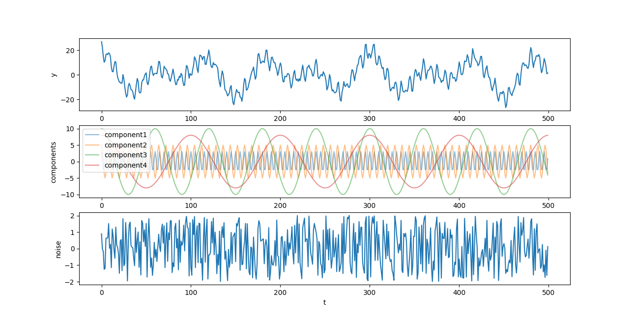
T1：构造时间序列

构造时间序列，至少包含五种成分和噪声，要求至少含有四个周期项$T1$、$T2$、$T3$和$T4$，要求$T1$和$T2$周期在同一尺度，$T3$大一个量级。

编写python代码如下：

import numpy as np
import matplotlib.pyplot as plt

# create data
T1 = 5
T2 = 8
T3 = 60
T4 = 100
x = np.arange(0, 500, 1)

def create_data(x):
    component1 = 3 * np.cos(2 * np.pi / T1 * x)
    component2 = 5 * np.cos(2 * np.pi / T2 * x)
    component3 = 10 * np.cos(2 * np.pi / T3 * x)
    component4 = 8 * np.cos(2 * np.pi / T4 * x)
    noise = np.random.uniform(-2, 2, len(x))
    all = component1 + component2 + component3 + component4 + noise
    return all, component1, component2, component3, component4, noise

y, y1, y2, y3, y4, noise = create_data(x)

# draw
ax1 = plt.subplot(311)
ax2 = plt.subplot(312)
ax3 = plt.subplot(313)
ax1.plot(x, y)
ax1.set_ylabel('y')
ax2.plot(x, y1, alpha=0.5, label='component1')
ax2.plot(x, y2, alpha=0.5, label='component2')
ax2.plot(x, y3, alpha=0.5, label='component3')
ax2.plot(x, y4, alpha=0.5, label='component4')
ax2.set_ylabel('components')
ax2.legend()
ax3.plot(x, noise)
ax3.set_ylabel('noise')
ax3.set_xlabel('t')
plt.show()

创建4个周期成分和一个均匀随机分布在 $[-2,2]$ 的噪声，并绘图得到

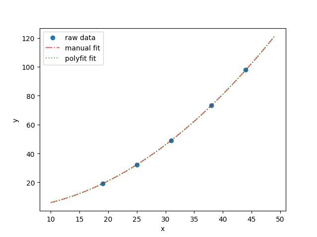
T2：最小二乘法拟合数据

用最小二乘法以 $y=a+b{x}^2$ 对数据进行拟合。

理论推导

待拟合数据 $(x_i,y_i),i=1,2,...,n$

要得到能使残差平方和 ${\displaystyle \mathrm{\Delta }=\sum _{i=1}^n{[y_i-(a+b{x}_i^2)]}^2}$ 最小的参数 $a,b$

将上式分别对参数 $a,b$ 求偏导：

$$\{\begin{array}{l}{\displaystyle \frac{\partial \mathrm{\Delta }}{\partial a}=-2\sum _{i=1}^n[y_i-(a+b{x}_i^2)]=0}\\ {\displaystyle \frac{\partial \mathrm{\Delta }}{\partial b}=-2\sum _{i=1}^n[y_i-(a+b{x}_i^2)]x_i^2=0}\end{array}$$

当 $a,b$ 满足上面偏导为零时，残差平方和 $\mathrm{\Delta }$ 取极小值，此时的 $a,b$ 记为最佳参数 $\hat{a},\hat{b}$ 。

上面二式化简为

$$\{\begin{array}{l}\hat{a}n+\hat{b}\sum x_i^2=\sum y_i\\ \hat{a}\sum x_i^2+\hat{b}\sum x_i^4=\sum x_i^2{y}_i\end{array}$$

解得

$$\{\begin{array}{l}{\displaystyle \hat{a}=\frac{\sum x_i^4\sum y_i-\sum x_i^2\sum x_i^2{y}_i}{n\sum x_i^4-(\sum x_i^2{)}^2}}\\ {\displaystyle \hat{b}=\frac{n\sum x_i^2{y}_i-\sum x_i^2\sum y_i}{n\sum x_i^4-(\sum x_i^2{)}^2}}\end{array}$$

编写程序

编写python代码如下：

import numpy as np
import matplotlib.pyplot as plt

# raw data
xi = np.array([19, 25, 31, 38, 44])
yi = np.array([19.0, 32.3, 49.0, 73.3, 97.8])

# find the least squares best fit line of the form y = a + bx^2
sum_x2 = 0
sum_x4 = 0
sum_y = 0
sum_x2y = 0
n = len(xi)
for i in range(n):
    sum_x2 += xi[i]**2
    sum_x4 += xi[i]**4
    sum_y += yi[i]
    sum_x2y += xi[i]**2 * yi[i]

a = (sum_x4 * sum_y - sum_x2y * sum_x2) / (n * sum_x4 - sum_x2**2)
b = (n * sum_x2y - sum_x2 * sum_y) / (n * sum_x4 - sum_x2**2)

x_fit = np.arange(10, 50, 1)
y_fit_manual = a + b * x_fit**2

# use polyfit to confirm
xi2 = xi**2
an = np.polyfit(xi2, yi, 1)
p = np.poly1d(an)
y_fit_polyfit = p(x_fit**2)

# draw
plt.scatter(xi, yi, label='raw data')
plt.plot(x_fit, y_fit_manual, 'r-.', alpha=0.6, label='manual fit')
plt.plot(x_fit, y_fit_polyfit, 'g:', alpha=0.6, label='polyfit fit')
plt.xlabel('x')
plt.ylabel('y')
plt.legend()
plt.show()

先使用理论推导中得到的参数公式进行计算，然后再用numpy模块自带的polyfit进行验证，绘图如下

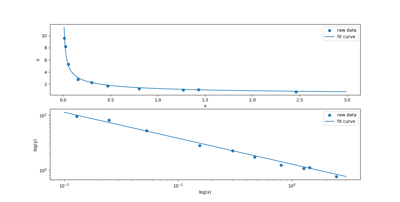
T3：曲线拟合并绘制对数图

用 $y=a{x}^c$ 进行拟合，并分别用线性尺度和对数尺度绘制拟合曲线图像。

编写python代码如下：

import numpy as np
import matplotlib.pyplot as plt
from scipy.optimize import curve_fit

# raw data
xi = np.array([0.0129, 0.0247, 0.053, 0.155, 0.301,
               0.471, 0.802, 1.27, 1.43, 2.46])
yi = np.array([9.56, 8.1845, 5.2616, 2.7917, 2.2611,
               1.734, 1.237, 1.0674, 1.1171, 0.762])

# use curve_fit to fit
def func(x, a, c):
    return a * x ** c

popt, pcov = curve_fit(func, xi, yi)
x_fit = np.arange(0, 3, 0.01)
y_fit = func(x_fit, popt[0], popt[1])

# draw
ax1 = plt.subplot(211)
ax1.scatter(xi, yi, label='raw data')
ax1.plot(x_fit, y_fit, label='fit curve')
ax1.set_xlabel('x')
ax1.set_ylabel('y')
ax1.legend()
ax2 = plt.subplot(212)
ax2.scatter(xi, yi, label='raw data')
ax2.plot(x_fit, y_fit, label='fit curve')
ax2.set_xscale('log')
ax2.set_yscale('log')
ax2.set_xlabel('log(x)')
ax2.set_ylabel('log(y)')
ax2.legend()
plt.show()

使用scipy模块中的curve_fit函数进行拟合，绘图如下