电动作业

作业

1. 推导绘制电偶极子的辐射场
2. 绘制电四极子辐射功率角分布
3. 绘制矩形孔的夫朗禾费衍射图样

1. 电偶极子辐射场

求电偶极子电场线方程

从矢势出发

$$\mathit{A}(\mathit{x})=\frac{{\mu }_0}{4\pi }{\int }_V\frac{\mathit{J}({\mathit{x}}^{\prime })e^{-ikr}}{r}\mathrm{d}{V}^{\prime }$$$$\mathit{B}=\mathrm{\nabla }\times \mathit{A}$$$$\begin{array}{rl}\mathit{E}& =-\frac{\partial \mathit{A}}{\partial t}-\mathrm{\nabla }\phi \\ & =-i\omega \mathit{A}+\frac{c^2\mathrm{\nabla }(\mathrm{\nabla }\cdot \mathit{A})}{i\omega }\end{array}$$

对电偶极子有

$$\mathit{A}=\frac{{\mu }_0\dot{p}}{4\pi r}{e}^{ikr}{\mathit{e}}_z$$$$\mathit{B}=\mathrm{\nabla }\times \mathit{A}=\frac{{\mu }_0\dot{p}}{4\pi r^2}{e}^{-ikr}(1+ikr)\sin \theta {\mathit{e}}_{\varphi }$$$$\Rightarrow \{\begin{array}{l}{E}_r=\sqrt{\frac{{\mu }_0}{{\epsilon }_0}}\frac{\dot{p}}{2\pi r^2}{e}^{-ikr}(1-\frac{i}{kr})\cos \theta \\ E_{\theta }=\sqrt{\frac{{\mu }_0}{{\epsilon }_0}}\frac{\dot{p}}{4\pi r^2}{e}^{-ikr}(1+ikr-\frac{i}{kr})\sin \theta \\ E_{\varphi }=0\end{array}$$

由电场线方程

$$\frac{\mathrm{d}r}{E_r}=\frac{r\mathrm{d}\theta }{E_{\varphi }}=\frac{r\sin \theta \mathrm{d}\varphi }{E_{\varphi }}$$$$\Rightarrow \frac{{\sin }^2\theta }{r}[kr\cos (\omega t-kr)+\sin (\omega t-kr)]=C$$

其中 $C$ 为积分常数，每一个 $C$ 对应一条电场线，取一组 $C$ 即为一族电场线。

绘制电场线

使用 python 绘制电场线并根据磁场方向填色

import numpy as np
import matplotlib.pyplot as plt
from matplotlib.animation import FuncAnimation

# set up the grid, parameters and colors
x = np.linspace(-30, 30, 601)
y = np.linspace(-30, 30, 601)
X, Y = np.meshgrid(x, y)
t_values = np.linspace(0, 20, 100)
C = [-0.9, -0.4, -0.1, 0, 0.1, 0.4, 0.9]
levels = [-2, -0.9, -0.4, -0.1, 0, 0.1, 0.4, 0.9, 2]
fill_colors_r = ['#ffffff', '#ffe09d', '#f5c57b', '#ebab5a', '#c5935d', '#847c83', '#4264a5', '#ffffff']
fill_colors_l = fill_colors_r[::-1]

# turn (x,y) into (R,Theta) and calculate E's equation
X = np.where(X == 0, 1e-6, X) # avoid division by zero
R = np.sqrt(X**2 + Y**2)
Theta = np.arctan2(Y, X) - np.pi / 2
def calc_E(t):
    E = np.sin(Theta)**2 / R * (R * np.cos(t - R) + np.sin(t - R))
    return E

# draw the curves E=C at each time t
fig, ax = plt.subplots(figsize=(8, 8))
def update(frame):
    ax.clear()
    t = t_values[frame]
    E = calc_E(t)
    ax.set_xlabel('x')
    ax.set_ylabel('y')
    ax.set_xlim(-30, 30)
    ax.set_ylim(-30, 30)
    ax.axis('equal')
    # draw the curves E=C
    ax.contour(X, Y, E, levels=C, colors='black', linewidths=0.5)
    # using colors to distinguish B's direction
    E_r = np.ma.masked_where(X >= 0, E)
    E_l = np.ma.masked_where(X < 0, E)
    ax.contourf(X, Y, E_r, levels=levels, colors=fill_colors_r, extend='both', antialiased=True)
    ax.contourf(X, Y, E_l, levels=levels, colors=fill_colors_l, extend='both', antialiased=True)
    return
update(0)
ani = FuncAnimation(fig, update, frames=len(t_values), interval=100, blit=False)
# ani.save('hw1_ed_animation.gif', writer='pillow')
plt.show()

绘图结果如下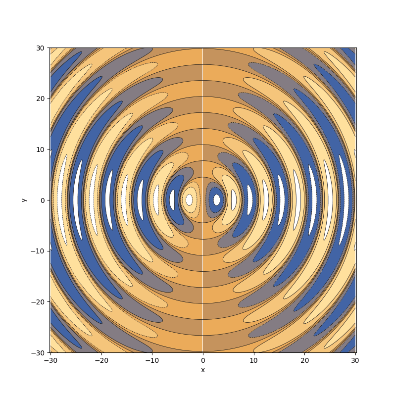

2. 电四极子辐射功率角分布

辐射功率角分布

辐射功率角分布因子

$$|\stackrel{⃛}{\overrightarrow{\mathcal{D}}}\times {\mathit{e}}_R{|}^2=36Q^2{l}^4{\omega }^6{\cos }^2\theta {\sin }^2\theta$$

绘制角分布图

用 python 绘制极坐标下 ${\cos }^2\theta {\sin }^2\theta$ 曲线

import numpy as np
import matplotlib.pyplot as plt

theta = np.linspace(0, 2 * np.pi, 1000)
r = np.cos(theta)**2 * np.sin(theta)**2

ax = plt.subplot(111, projection='polar')
ax.plot(theta, r)
plt.show()

结果如下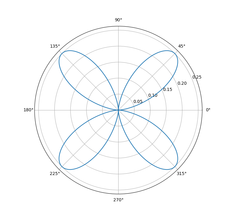

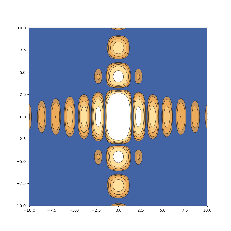
3. 矩形孔的夫朗禾费衍射

矩形孔的夫朗禾费衍射光强分布

光强分布

$$I=I_0{\left(\frac{\sin ka\alpha }{ka\alpha }\right)}^2{\left(\frac{\sin kb\beta }{kb\beta }\right)}^2$$

其中 $\alpha =\arcsin \frac{x}{d}\approx \frac{x}{d},\beta =\arcsin \frac{y}{d}\approx \frac{y}{d}$

绘制光强分布图

用 python 绘制 $I$ 的等高线图并填色

import numpy as np
import matplotlib.pyplot as plt

x = np.linspace(-10, 10, 400)
y = np.linspace(-10, 10, 400)
X, Y = np.meshgrid(x, y)

a, b = 2, 1
d = 100
k = 100
alpha = X / d
beta = Y / d
Z = (np.sin(k*a*alpha)/(k*a*alpha))**2 * (np.sin(k*b*beta)/(k*b*beta))**2

levels = [0.001, 0.002, 0.005, 0.01, 0.03]
fill_colors = ['#4264a5', '#c5935d', '#ebab5a', '#f5c57b', '#ffe09d', '#ffffff']

plt.figure(figsize=(8, 8))
plt.contour(X, Y, Z, levels=levels, colors='black', linewidths=0.5)
plt.contourf(X, Y, Z, levels=levels, colors=fill_colors, extend='both', antialiased=True)
plt.axis('equal')
plt.show()

绘图结果如下