Dias, F., & Bridges, T. (2005). Weakly nonlinear wave packets and the nonlinear Schrödinger equation. In R. Grimshaw (Ed.), Nonlinear waves in fluids: Recent advances and modern applications (pp. 29–67). Springer. https://doi.org/10.1007/3-211-38025-6_2
The method of multiple scales
A derivation of the NLS (nonlinear Schrödinger) equation from the KdV (Korteweg-de Vries) equation based on the method of multiple scales.
The KdV equation
L ( u ) + N ( u , u ) = u t + u x x x + 6 u u x = 0 , ( x ∈ R , t ≥ 0 , u ( x , t ) ∈ R ) . \mathcal{L}(u)+\mathcal{N}(u,u)=u_t+u_{xxx}+6uu_x=0,\quad(x\in\mathbb{R},t\ge0,u(x,t)\in\mathbb{R}).
L ( u ) + N ( u , u ) = u t + u xxx + 6 u u x = 0 , ( x ∈ R , t ≥ 0 , u ( x , t ) ∈ R ) .
Introducting a small parameter ϵ \epsilon ϵ X = ϵ x , T = ϵ t , τ = ϵ 2 t X=\epsilon x,T=\epsilon t,\tau=\epsilon^2 t X = ϵ x , T = ϵ t , τ = ϵ 2 t
u = ϵ ( u 0 + ϵ u 1 + ϵ 2 u 2 + ⋯ ) = ϵ u 0 + ϵ 2 u 1 + ϵ 3 u 2 + ⋯ , u=\epsilon(u_0+\epsilon u_1+\epsilon^2 u_2+\cdots)=\epsilon u_0+\epsilon^2 u_1+\epsilon^3 u_2+\cdots,
u = ϵ ( u 0 + ϵ u 1 + ϵ 2 u 2 + ⋯ ) = ϵ u 0 + ϵ 2 u 1 + ϵ 3 u 2 + ⋯ ,
L = ∂ t + ∂ x x x = ( ∂ ∂ t + ϵ ∂ ∂ T + ϵ 2 ∂ ∂ τ ) + ( ∂ ∂ x + ϵ ∂ ∂ X ) 3 = ( ∂ ∂ t + ∂ 3 ∂ x 3 ) + ϵ ( ∂ ∂ T + 3 ∂ 3 ∂ x 2 ∂ X ) + ϵ 2 ( ∂ ∂ τ + 3 ∂ 3 ∂ x ∂ X 2 ) + ⋯ ≡ L ( 0 ) + ϵ L ( 1 ) + ϵ 2 L ( 2 ) + ⋯ , \begin{aligned}
\mathcal{L}&=\partial_t+\partial_{xxx} \\
&=\left(\frac{\partial}{\partial t}+\epsilon\frac{\partial}{\partial T}+\epsilon^2\frac{\partial}{\partial \tau}\right)+\left(\frac{\partial}{\partial x}+\epsilon\frac{\partial}{\partial X}\right)^3 \\
&=\left(\frac{\partial}{\partial t}+\frac{\partial^3}{\partial x^3}\right)+\epsilon\left(\frac{\partial}{\partial T}+3\frac{\partial^3}{\partial x^2\partial X}\right)+\epsilon^2\left(\frac{\partial}{\partial\tau}+3\frac{\partial^3}{\partial x\partial X^2}\right)+\cdots \\
&\equiv\mathcal{L}^{(0)}+\epsilon\mathcal{L}^{(1)}+\epsilon^2\mathcal{L}^{(2)}+\cdots,
\end{aligned}
L = ∂ t + ∂ xxx = ( ∂ t ∂ + ϵ ∂ T ∂ + ϵ 2 ∂ τ ∂ ) + ( ∂ x ∂ + ϵ ∂ X ∂ ) 3 = ( ∂ t ∂ + ∂ x 3 ∂ 3 ) + ϵ ( ∂ T ∂ + 3 ∂ x 2 ∂ X ∂ 3 ) + ϵ 2 ( ∂ τ ∂ + 3 ∂ x ∂ X 2 ∂ 3 ) + ⋯ ≡ L ( 0 ) + ϵ L ( 1 ) + ϵ 2 L ( 2 ) + ⋯ ,
O ( ϵ ) L ( 0 ) u 0 = 0 , O ( ϵ 2 ) L ( 0 ) u 1 = − L ( 1 ) u 0 − 3 ∂ x ( u 0 2 ) , O ( ϵ 3 ) L ( 0 ) u 2 = − L ( 2 ) u 0 − L ( 1 ) u 1 − 6 ∂ x ( u 0 u 1 ) − 3 ∂ X ( u 0 2 ) . \begin{array}{ll}
\mathcal{O}(\epsilon) & \mathcal{L}^{(0)}u_0=0, \\
\mathcal{O}(\epsilon^2) & \mathcal{L}^{(0)}u_1=-\mathcal{L}^{(1)}u_0-3\partial_x(u_0^2), \\
\mathcal{O}(\epsilon^3) & \mathcal{L}^{(0)}u_2=-\mathcal{L}^{(2)}u_0-\mathcal{L}^{(1)}u_1-6\partial_x(u_0u_1)-3\partial_X(u_0^2).
\end{array}
O ( ϵ ) O ( ϵ 2 ) O ( ϵ 3 ) L ( 0 ) u 0 = 0 , L ( 0 ) u 1 = − L ( 1 ) u 0 − 3 ∂ x ( u 0 2 ) , L ( 0 ) u 2 = − L ( 2 ) u 0 − L ( 1 ) u 1 − 6 ∂ x ( u 0 u 1 ) − 3 ∂ X ( u 0 2 ) .
At O ( ϵ ) \mathcal{O}(\epsilon) O ( ϵ ) L ( 0 ) u 0 = 0 \mathcal{L}^{(0)}u_0=0 L ( 0 ) u 0 = 0
u 0 ( x , t ) = ψ 0 ( X , T ) exp [ i ( k x − ω t ) ] + c.c. u_0(x,t)=\psi_0(X,T)\exp[i(kx-\omega t)]+\text{c.c.}
u 0 ( x , t ) = ψ 0 ( X , T ) exp [ i ( k x − ω t )] + c.c.
with the dispersion relation (decided by the linear operator L ( 0 ) \mathcal{L}^{(0)} L ( 0 )
ω = − k 3 . \omega=-k^3.
ω = − k 3 .
the phase velocity c = ω / k c=\omega/k c = ω / k c g = d ω / d k = − 3 k 2 c_g=\mathrm{d}\omega/\mathrm{d}k=-3k^2 c g = d ω / d k = − 3 k 2
At O ( ϵ 2 ) \mathcal{O}(\epsilon^2) O ( ϵ 2 ) L ( 0 ) u 1 = − L ( 1 ) u 0 − 3 ∂ x ( u 0 2 ) \mathcal{L}^{(0)}u_1=-\mathcal{L}^{(1)}u_0-3\partial_x(u_0^2) L ( 0 ) u 1 = − L ( 1 ) u 0 − 3 ∂ x ( u 0 2 )
L ( 1 ) u 0 = 0 ⇒ ( ∂ T + c g ∂ X ) u 0 = 0 \mathcal{L}^{(1)}u_0=0\Rightarrow(\partial_T+c_g\partial_X)u_0=0
L ( 1 ) u 0 = 0 ⇒ ( ∂ T + c g ∂ X ) u 0 = 0
on the time scale T T T ξ = X − c g T \xi=X-c_gT ξ = X − c g T
choose the function
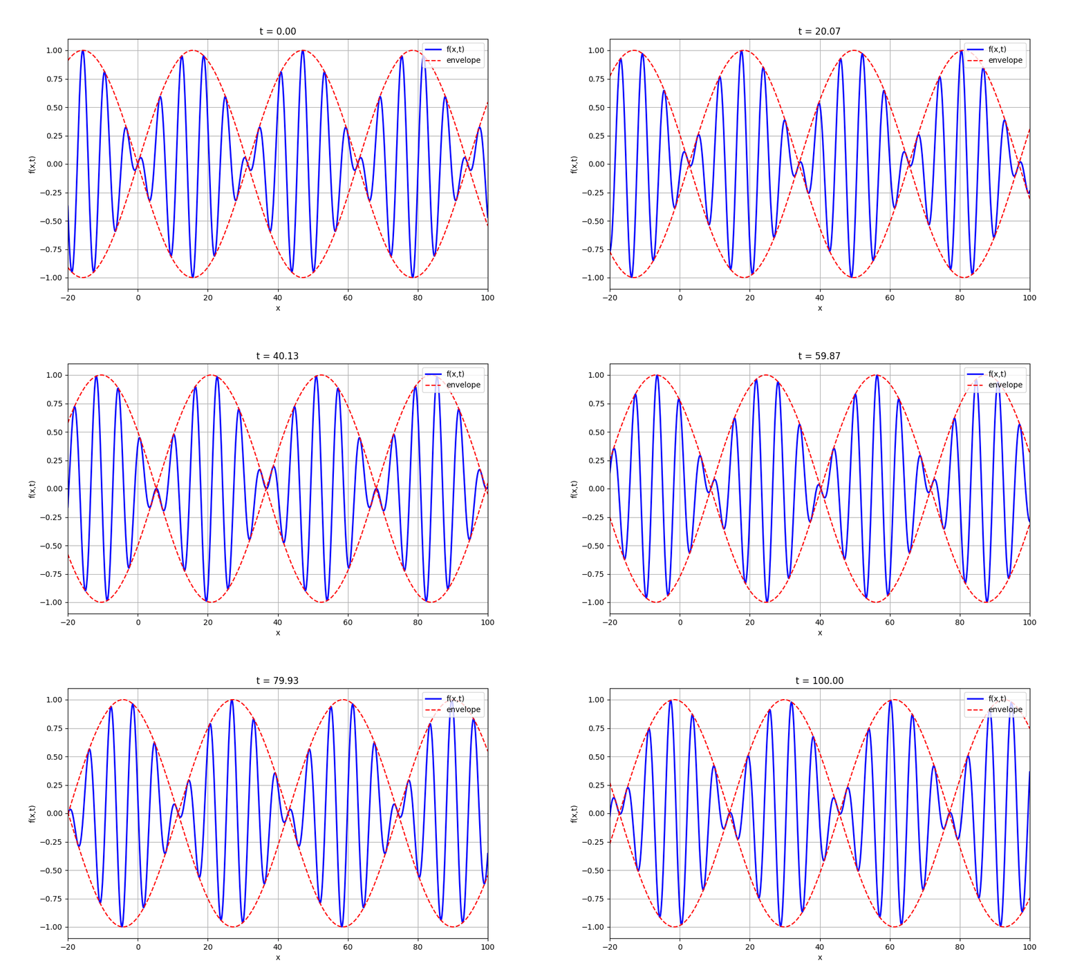
f ( x , t ) = ψ ( X , T ) cos ( k x − ω t ) = ψ ( X − c g T ) cos ( k x − ω t ) = sin [ ϵ ( x − c g t ) ] cos ( k x − ω t ) = sin [ ϵ ( x + 3 k 2 t ) ] cos ( k x + k 3 t ) \begin{aligned} f(x,t)&=\psi(X,T)\cos(kx-\omega t) \\ &=\psi(X-c_g T)\cos(kx-\omega t) \\ &=\sin[\epsilon(x-c_g t)]\cos(kx-\omega t) \\ &=\sin[\epsilon(x+3k^2 t)]\cos(kx+k^3 t) \end{aligned} f ( x , t ) = ψ ( X , T ) cos ( k x − ω t ) = ψ ( X − c g T ) cos ( k x − ω t ) = sin [ ϵ ( x − c g t )] cos ( k x − ω t ) = sin [ ϵ ( x + 3 k 2 t )] cos ( k x + k 3 t )
set ϵ = 0.1 , k = 1 \epsilon=0.1, k=1 ϵ = 0.1 , k = 1 ω = − k 3 = − 1 \omega=-k^3=-1 ω = − k 3 = − 1 c = ω / k = − 1 c=\omega/k=-1 c = ω / k = − 1 c g = d ω / d k = − 3 k 2 = − 3 c_g=\mathrm{d}\omega/\mathrm{d}k=-3k^2=-3 c g = d ω / d k = − 3 k 2 = − 3
1
2
3
4
5
6
7
8
9
10
11
12
13
14
15
16
17
18
19
20
21
22
23
24
25
26
27
28
29
30
31
32
33
34
35
36
37
38
39
40
41
42
43
44
45
46
47
48
49
50
51
52
53
54
55
56
57
58
59
60
61
62
import numpy as npimport matplotlib.pyplot as pltfrom matplotlib.animation import FuncAnimation0.1 1.0 20 , 100 , 1000 )0 , 100 , 300 )10 , 6 ))20 , 100 )1.1 , 1.1 )'x' )'f(x,t)' )True )'b-' , lw=2 , label='f(x,t)' )'r--' , lw=1.5 , label='envelope' )'r--' , lw=1.5 )'upper right' , bbox_to_anchor=(1.0 , 1.0 ), frameon=True )def init ():return line_f, line_env_pos, line_env_negdef update (frame ):3 * k**2 * t)) * np.cos(k * x + k**3 * t)3 * k**2 * t))f't = {t:.2 f} ' )return line_f, line_env_pos, line_env_neglen (t_frames), init_func=init,True , interval=50 )'wave_animation.gif' , writer='ffmpeg' , fps=20 )
Then solve for u 1 u_1 u 1
L ( 0 ) u 1 = − 3 ∂ x ( ϕ 0 2 e 2 i ( k x − ω t ) + c.c. ) (2.10) \mathcal{L}^{(0)}u_1=-3\partial_x(\phi_0^2e^{2i(kx-\omega t)}+\text{c.c.})\tag{2.10}
L ( 0 ) u 1 = − 3 ∂ x ( ϕ 0 2 e 2 i ( k x − ω t ) + c.c. ) ( 2.10 )
the general solution is
u 1 = A 2 ( X , T ) e 2 i ( k x − ω t ) + c.c. + ψ 1 e i ( k x − ω t ) + c.c. + A 0 ( X , T ) u_1=A_2(X,T)e^{2i(kx-\omega t)}+\text{c.c.}+\psi_1 e^{i(kx-\omega t)}+\text{c.c.}+A_0(X,T)
u 1 = A 2 ( X , T ) e 2 i ( k x − ω t ) + c.c. + ψ 1 e i ( k x − ω t ) + c.c. + A 0 ( X , T )
the term ψ 1 e i ( k x − ω t ) \psi_1 e^{i(kx-\omega t)} ψ 1 e i ( k x − ω t ) ψ 0 e i ( k x − ω t ) \psi_0 e^{i(kx-\omega t)} ψ 0 e i ( k x − ω t ) ψ = ψ 0 + ϵ ψ 1 \psi=\psi_0+\epsilon\psi_1 ψ = ψ 0 + ϵ ψ 1
{ u 0 = ψ e i ( k x − ω t ) + c.c. , u 1 = A 2 ( X , T ) e 2 i ( k x − ω t ) + c.c. + A 0 ( X , T ) , \left\{
\begin{aligned}
u_0&=\psi e^{i(kx-\omega t)}+\text{c.c.}, \\
u_1&=A_2(X,T)e^{2i(kx-\omega t)}+\text{c.c.}+A_0(X,T),
\end{aligned}
\right.
{ u 0 u 1 = ψ e i ( k x − ω t ) + c.c. , = A 2 ( X , T ) e 2 i ( k x − ω t ) + c.c. + A 0 ( X , T ) ,
u 1 → O ( ϵ 2 ) (2.10) ⇒ A 2 = − 3 ( 2 i k ) ψ 2 − 2 i ω + ( 2 i k ) 3 = ψ 2 k 2 . u_1\rightarrow\mathcal{O}(\epsilon^2)\text{(2.10)}\Rightarrow A_2=\frac{-3(2ik)\psi^2}{-2i\omega+(2ik)^3}=\frac{\psi^2}{k^2}.
u 1 → O ( ϵ 2 ) (2.10) ⇒ A 2 = − 2 iω + ( 2 ik ) 3 − 3 ( 2 ik ) ψ 2 = k 2 ψ 2 .
At O ( ϵ 3 ) \mathcal{O}(\epsilon^3) O ( ϵ 3 ) L ( 0 ) u 2 = − L ( 2 ) u 0 − L ( 1 ) u 1 − 6 ∂ x ( u 0 u 1 ) − 3 ∂ X ( u 0 2 ) \mathcal{L}^{(0)}u_2=-\mathcal{L}^{(2)}u_0-\mathcal{L}^{(1)}u_1-6\partial_x(u_0u_1)-3\partial_X(u_0^2) L ( 0 ) u 2 = − L ( 2 ) u 0 − L ( 1 ) u 1 − 6 ∂ x ( u 0 u 1 ) − 3 ∂ X ( u 0 2 )
− ∂ τ ψ − 3 i k ∂ X X ψ − 6 i k ∣ ψ ∣ 2 ψ / k − 6 i k A 0 ψ = 0 (2.13) -\partial_\tau\psi-3ik\partial_{XX}\psi-6ik|\psi|^2\psi/k-6ikA_0\psi=0\tag{2.13}
− ∂ τ ψ − 3 ik ∂ X X ψ − 6 ik ∣ ψ ∣ 2 ψ / k − 6 ik A 0 ψ = 0 ( 2.13 )
Equating the coefficients of the oscillation free (time average) terms in (2.13)
− ∂ T A 0 − 6 ∂ X ∣ ψ ∣ 2 = 0 ⇒ A 0 = − 2 ∣ ψ ∣ 2 k 2 -\partial_T A_0-6\partial_X|\psi|^2=0\Rightarrow A_0=-\frac{2|\psi|^2}{k^2}
− ∂ T A 0 − 6 ∂ X ∣ ψ ∣ 2 = 0 ⇒ A 0 = − k 2 2∣ ψ ∣ 2
noting that d 2 ω / d k 2 = − 6 k \mathrm{d}^2\omega/\mathrm{d}k^2=-6k d 2 ω / d k 2 = − 6 k
i ∂ ψ ∂ τ + 1 2 d 2 ω d k 2 ∂ 2 ψ ∂ ξ 2 + 6 k ∣ ψ ∣ 2 ψ = 0. i\frac{\partial\psi}{\partial\tau}+\frac{1}{2}\frac{\mathrm{d}^2\omega}{\mathrm{d}k^2}\frac{\partial^2\psi}{\partial\xi^2}+\frac{6}{k}|\psi|^2\psi=0.
i ∂ τ ∂ ψ + 2 1 d k 2 d 2 ω ∂ ξ 2 ∂ 2 ψ + k 6 ∣ ψ ∣ 2 ψ = 0.
The water-wave problem
The governing equations:Δ ϕ = 0 \Delta \phi=0 Δ ϕ = 0 u = ∇ ϕ ( x , y , z , t ) \boldsymbol{u}=\nabla\phi(x,y,z,t) u = ∇ ϕ ( x , y , z , t ) ∂ ϕ ∂ t + 1 2 ∣ ∇ ϕ ∣ 2 + g z + p − p 0 ρ = 0. \frac{\partial\phi}{\partial t}+\frac{1}{2}|\nabla\phi|^2+gz+\frac{p-p_0}{\rho}=0.
∂ t ∂ ϕ + 2 1 ∣∇ ϕ ∣ 2 + g z + ρ p − p 0 = 0.
The flow domain:F ( x , y , z , t ) ≡ η ( x , y , t ) − z = 0 F(x,y,z,t)\equiv\eta(x,y,t)-z=0 F ( x , y , z , t ) ≡ η ( x , y , t ) − z = 0 z = − h z=-h z = − h
Boundary conditions:D F / D t = 0 ⇒ DF/Dt=0\Rightarrow D F / D t = 0 ⇒ η t + ϕ x η x + ϕ y η y − ϕ z = 0 \eta_t+\phi_x\eta_x+\phi_y\eta_y-\phi_z=0 η t + ϕ x η x + ϕ y η y − ϕ z = 0 ϕ t + 1 2 ( ϕ x 2 + ϕ y 2 + ϕ z 2 ) + g η − σ ρ C = 0 \phi_t+\frac{1}{2}\left(\phi_x^2+\phi_y^2+\phi_z^2\right)+g\eta-\frac{\sigma}{\rho}C=0
ϕ t + 2 1 ( ϕ x 2 + ϕ y 2 + ϕ z 2 ) + g η − ρ σ C = 0
where C C C ϕ z ( x , y , − h , t ) = 0 \phi_z(x,y,-h,t)=0 ϕ z ( x , y , − h , t ) = 0
To summarize, solve for η ( x , y , t ) \eta(x,y,t) η ( x , y , t ) ϕ ( x , y , z , t ) \phi(x,y,z,t) ϕ ( x , y , z , t )
Δ ϕ ≡ ϕ x x + ϕ y y + ϕ z z = 0 , for ( x , y , z ) ∈ R × R × [ − h , η ] , η t + ϕ x η x + ϕ y η y − ϕ z = 0 , on z = η ( x , y , t ) , ϕ t + 1 2 ( ϕ x 2 + ϕ y 2 + ϕ z 2 ) + g η − σ ρ C = 0 , on z = η ( x , y , t ) , ϕ z = 0 , on z = − h \begin{aligned}
\Delta\phi\equiv\phi_{xx}+\phi_{yy}+\phi_{zz}&=0,\text{ for }(x,y,z)\in\mathbb{R}\times\mathbb{R}\times[-h,\eta], \\
\eta_t+\phi_x\eta_x+\phi_y\eta_y-\phi_z&=0,\text{ on }z=\eta(x,y,t), \\
\phi_t+\frac{1}{2}\left(\phi_x^2+\phi_y^2+\phi_z^2\right)+g\eta-\frac{\sigma}{\rho}C&=0,\text{ on }z=\eta(x,y,t), \\
\phi_z&=0,\text{ on }z=-h
\end{aligned}
Δ ϕ ≡ ϕ xx + ϕ y y + ϕ z z η t + ϕ x η x + ϕ y η y − ϕ z ϕ t + 2 1 ( ϕ x 2 + ϕ y 2 + ϕ z 2 ) + g η − ρ σ C ϕ z = 0 , for ( x , y , z ) ∈ R × R × [ − h , η ] , = 0 , on z = η ( x , y , t ) , = 0 , on z = η ( x , y , t ) , = 0 , on z = − h
Linearization of the 2D problem
Looks for solutions which are periodic in x x x k k k t t t ω \omega ω
( x ∗ , z ∗ ) = ( k x , k z ) , η ∗ = η a , t ∗ = ω t , ϕ ∗ = k ω a ϕ , (x^*,z^*)=(kx,kz),\quad\eta^*=\frac{\eta}{a},\quad t^*=\omega t,\quad\phi^*=\frac{k}{\omega a}\phi,
( x ∗ , z ∗ ) = ( k x , k z ) , η ∗ = a η , t ∗ = ω t , ϕ ∗ = ω a k ϕ ,
where a a a
Dropping the stars, the surface wave problem linearized around the equilibrium state η = 0 , u = 0 \eta=0,\boldsymbol{u}=\boldsymbol{0} η = 0 , u = 0
ϕ x x + ϕ z z = 0 , for ( x , z ) ∈ R × [ − k h , 0 ] , η t − ϕ z = 0 , on z = 0 , ϕ t + ( g k ω 2 ) η − ( σ k 3 ρ ω 2 ) η x x = 0 , on z = 0 , ϕ z = 0 , on z = − k h \begin{aligned}
\phi_{xx}+\phi_{zz}&=0,\text{ for }(x,z)\in\mathbb{R}\times[-kh,0], \\
\eta_t-\phi_z&=0,\text{ on }z=0, \\
\phi_t+\left(\frac{gk}{\omega^2}\right)\eta-\left(\frac{\sigma k^3}{\rho\omega^2}\right)\eta_{xx}&=0,\text{ on }z=0, \\
\phi_z&=0,\text{ on }z=-kh
\end{aligned}
ϕ xx + ϕ z z η t − ϕ z ϕ t + ( ω 2 g k ) η − ( ρ ω 2 σ k 3 ) η xx ϕ z = 0 , for ( x , z ) ∈ R × [ − k h , 0 ] , = 0 , on z = 0 , = 0 , on z = 0 , = 0 , on z = − k h
assume η ( x , t ) = cos ( x − t + Θ ) \eta(x,t)=\cos(x-t+\Theta) η ( x , t ) = cos ( x − t + Θ )
ϕ ( x − t , z ) = 1 tanh ( k h ) sin ( x − t + Θ ) cosh ( z + k h ) cos ( k h ) \phi(x-t,z)=\frac{1}{\tanh(kh)}\sin(x-t+\Theta)\frac{\cosh(z+kh)}{\cos(kh)}
ϕ ( x − t , z ) = tanh ( k h ) 1 sin ( x − t + Θ ) cos ( k h ) cosh ( z + k h )
and the dynamic condition yields the dispersion relation for linearized 2D capillary-gravity periodic waves in water of finite depth
ω 2 − g k tanh ( k h ) ( 1 + σ k 2 ρ g ) = 0. \omega^2-gk\tanh(kh)\left(1+\frac{\sigma k^2}{\rho g}\right)=0.
ω 2 − g k tanh ( k h ) ( 1 + ρ g σ k 2 ) = 0.
Interpretation of the group velocity:
the travel velocity of the envelope;
the speed of propagation of energy.
For 3D waves
The extension of the dispersion relation to three-dimensional waves is
ω 2 − g ∣ k ∣ tanh ( ∣ k h ∣ ) ( 1 + σ ∣ k ∣ 2 ρ g ) = 0 \omega^2-g|\boldsymbol{k}|\tanh(|\boldsymbol{k}h|)\left(1+\frac{\sigma|\boldsymbol{k}|^2}{\rho g}\right)=0
ω 2 − g ∣ k ∣ tanh ( ∣ k h ∣ ) ( 1 + ρ g σ ∣ k ∣ 2 ) = 0
where ∣ k ∣ = k 2 + l 2 |\boldsymbol{k}|=\sqrt{k^2+l^2} ∣ k ∣ = k 2 + l 2
The common ansatz used in the multiple scales:
η = ∑ n = 1 3 ϵ n η n ( x 0 , x 1 , x 2 ; y 1 , y 2 ; t 0 , t 1 , t 2 ) + O ( ϵ 4 ) , ϕ = ∑ n = 1 3 ϵ n ϕ n ( x 0 , x 1 , x 2 ; y 1 , y 2 ; z ; t 0 , t 1 , t 2 ) + O ( ϵ 4 ) \begin{aligned}
\eta &=\sum_{n=1}^3 \epsilon^n\eta_n(x_0,x_1,x_2;y_1,y_2;t_0,t_1,t_2)+\mathcal{O}(\epsilon^4), \\
\phi &=\sum_{n=1}^3 \epsilon^n\phi_n(x_0,x_1,x_2;y_1,y_2;z;t_0,t_1,t_2)+\mathcal{O}(\epsilon^4)
\end{aligned}
η ϕ = n = 1 ∑ 3 ϵ n η n ( x 0 , x 1 , x 2 ; y 1 , y 2 ; t 0 , t 1 , t 2 ) + O ( ϵ 4 ) , = n = 1 ∑ 3 ϵ n ϕ n ( x 0 , x 1 , x 2 ; y 1 , y 2 ; z ; t 0 , t 1 , t 2 ) + O ( ϵ 4 )
where
x 0 = x , x 1 = ϵ x , x 2 = ϵ 2 x , y 1 = ϵ y , y 2 = ϵ 2 y , t 0 = t , t 1 = ϵ t , t 2 = ϵ 2 t . \begin{array}{lll}
x_0=x, & x_1=\epsilon x, & x_2=\epsilon^2 x, \\
& y_1=\epsilon y, & y_2=\epsilon^2 y, \\
t_0=t, & t_1=\epsilon t, & t_2=\epsilon^2 t.
\end{array}
x 0 = x , t 0 = t , x 1 = ϵ x , y 1 = ϵy , t 1 = ϵ t , x 2 = ϵ 2 x , y 2 = ϵ 2 y , t 2 = ϵ 2 t .
The order one component of η \eta η
η 1 = A e i ( k x − ω t ) + c.c. \eta_1=Ae^{i(kx-\omega t)}+\text{c.c.}
η 1 = A e i ( k x − ω t ) + c.c.
Applying the method of multiple scales, the solvability condition at O ( ϵ 3 ) \mathcal{O}(\epsilon^3) O ( ϵ 3 ) A A A
2 i ∂ A ∂ t 2 + p ∂ 2 A ∂ ξ 2 + q ∂ 2 A ∂ y 1 2 + γ A ∣ A ∣ 2 = − i ϵ ( s A ξ y 1 y 1 + r A ξ ξ ξ + u A 2 A ξ ∗ − v ∣ A ∣ 2 A ξ ) + ϵ A ϕ ˉ ξ ∣ z 1 = 0 . \begin{aligned}
2i\frac{\partial A}{\partial t_2}+p\frac{\partial^2 A}{\partial \xi^2}+q\frac{\partial^2 A}{\partial y_1^2}+\gamma A|A|^2={}&-i\epsilon(sA_{\xi y_1y_1}+rA_{\xi\xi\xi}+uA^2A^*_\xi-v|A|^2A_\xi) \\
&+\epsilon A\left.\bar{\phi}_\xi\right|_{z_1=0}.
\end{aligned}
2 i ∂ t 2 ∂ A + p ∂ ξ 2 ∂ 2 A + q ∂ y 1 2 ∂ 2 A + γ A ∣ A ∣ 2 = − i ϵ ( s A ξ y 1 y 1 + r A ξ ξ ξ + u A 2 A ξ ∗ − v ∣ A ∣ 2 A ξ ) + ϵ A ϕ ˉ ξ z 1 = 0 .
The NLS equation:
i u t + α u x x + γ ∣ u ∣ 2 u = 0 , u ∈ C . iu_t+\alpha u_{xx}+\gamma|u|^2u=0,\quad u\in\mathbb{C}. i u t + α u xx + γ ∣ u ∣ 2 u = 0 , u ∈ C .
 ▶python script