Table of contents

Introduction

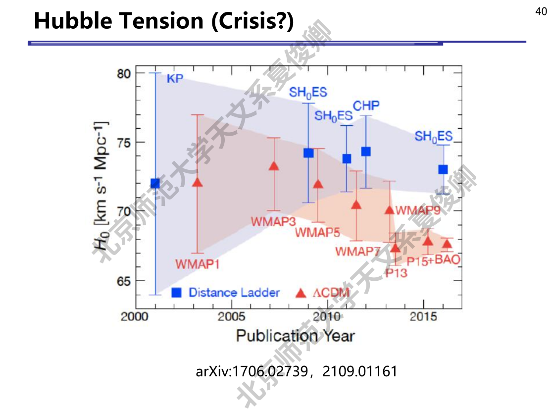
Hubble Tension

CMB v.s. Supernova

The spatial curvature of the Universe

Methodology

Traditional Method

• model

$\Lambda$CDM

• Friedman equation
• theoretical angular diameter distance $D_A^{\text{th}}(z;\boldsymbol{p})$
• get observed distance $D_A^{\text{obs}}(z)$
• obtain cosmological parameters $\boldsymbol{p}$ by chi-square-minimized (Markov Chain Monte Carlo method)

Traditional Method

• model
• Friedman equation

$$ E(z)\equiv\left(\frac{H(z)}{H_0}\right)^2=\Omega_{m}(1+z)^3+\Omega_{k}(1+z)^2+\Omega_{\Lambda} $$

• theoretical angular diameter distance $D_A^{\text{th}}(z;\boldsymbol{p})$
• get observed distance $D_A^{\text{obs}}(z)$
• obtain cosmological parameters $\boldsymbol{p}$ by chi-square-minimized (Markov Chain Monte Carlo method)

Traditional Method

• model
• Friedman equation

$$ E(z)\equiv\left(\frac{H(z)}{H_0}\right)^2=\Omega_{m}(1+z)^3+\Omega_{k}(1+z)^2+\Omega_{\Lambda} $$

• theoretical angular diameter distance $D_A^{\text{th}}(z;\boldsymbol{p})$

$$ D_A^{\text{th}}(z;\boldsymbol{p})=\left\{\begin{array}{ll} \displaystyle\frac{D_H}{(1+z)\sqrt{|\Omega_k}|}\sinh^{-1}\left(\sqrt{|\Omega_k|}\int_0^z\frac{\mathrm{d}z'}{E(z')^{1/2}}\right) & \text{for}\ \Omega_k>0 \\ \displaystyle\frac{D_H}{(1+z)}\int\frac{\mathrm{d}z'}{E(z')^{1/2}} & \text{for}\ \Omega_k=0 \\ \displaystyle\frac{D_H}{(1+z)\sqrt{|\Omega_k}|}\sin^{-1}\left(\sqrt{|\Omega_k|}\int_0^z\frac{\mathrm{d}z'}{E(z')^{1/2}}\right) & \text{for}\ \Omega_k<0 \\ \end{array}\right. $$ here $\boldsymbol{p}=(\Omega_m,\Omega_k,\Omega_\Lambda)$

• get observed distance $D_A^{\text{obs}}(z)$
• obtain cosmological parameters $\boldsymbol{p}$ by chi-square-minimized (Markov Chain Monte Carlo method)

Traditional Method

• model
• Friedman equation
• theoretical angular diameter distance $D_A^{\text{th}}(z;\boldsymbol{p})$
• get observed distance $D_A^{\text{obs}}(z)$
• obtain cosmological parameters $\boldsymbol{p}$ by chi-square-minimized (Markov Chain Monte Carlo method)

This work

• gravitational wave (GW)'s phase shift
• acceleration parameter $X(z)$($H(z)$)
• using artificial neural network (ANN) to get function ($z\rightarrow X(z)$)
• theoretical angular diameter distance $D_A^{\text{th}}(z;\boldsymbol{p})$
• get observed distance $D_A^{\text{obs}}(z)$
• obtain cosmological parameters $\boldsymbol{p}$ by chi-square-minimized (Markov Chain Monte Carlo method)

This work

• gravitational wave (GW)'s phase shift
• acceleration parameter $X(z)$($H(z)$)

$$ X(z)\equiv\frac{H_0}{2}\left(1-\frac{H(z)}{(1+z)H_0}\right) $$

• using artificial neural network (ANN) to get function ($z\rightarrow X(z)$)
• theoretical angular diameter distance $D_A^{\text{th}}(z;\boldsymbol{p})$
• get observed distance $D_A^{\text{obs}}(z)$
• obtain cosmological parameters $\boldsymbol{p}$ by chi-square-minimized (Markov Chain Monte Carlo method)

This work

• gravitational wave (GW)'s phase shift
• acceleration parameter $X(z)$($H(z)$)

$$ X(z)\equiv\frac{H_0}{2}\left(1-\frac{H(z)}{(1+z)H_0}\right) $$

• using artificial neural network (ANN) to get function ($z\rightarrow X(z)$)
• theoretical angular diameter distance $D_A^{\text{th}}(z;\boldsymbol{p})$

$$ D_A^{\text{th}}(z;\boldsymbol{p})=\left\{\begin{array}{ll} \displaystyle\frac{D_H}{(1+z)\sqrt{|\Omega_k}|}\sinh^{-1}\left(\sqrt{|\Omega_k|}\frac{H_0}{1+z}\int_0^z\frac{\mathrm{d}z'}{H_0-2X(z')}\right) & \text{for}\ \Omega_k>0 \\ \displaystyle\frac{c}{(1+z)^2}\int\frac{\mathrm{d}z'}{H_0-2X(z')} & \text{for}\ \Omega_k=0 \\ \displaystyle\frac{D_H}{(1+z)\sqrt{|\Omega_k}|}\sin^{-1}\left(\sqrt{|\Omega_k|}\frac{H_0}{1+z}\int_0^z\frac{\mathrm{d}z'}{H_0-2X(z')}\right) & \text{for}\ \Omega_k>0 \\ \end{array}\right. $$ here $\boldsymbol{p}=(H_0,\Omega_k)$

• get observed distance $D_A^{\text{obs}}(z)$
• obtain cosmological parameters $\boldsymbol{p}$ by chi-square-minimized (Markov Chain Monte Carlo method)

This work

• gravitational wave (GW)'s phase shift
• acceleration parameter $X(z)$($H(z)$)
• using artificial neural network (ANN) to get function ($z\rightarrow X(z)$)
• theoretical angular diameter distance $D_A^{\text{th}}(z;\boldsymbol{p})$
• get observed distance $D_A^{\text{obs}}(z)$
• obtain cosmological parameters $\boldsymbol{p}$ by chi-square-minimized (Markov Chain Monte Carlo method)

GW $\rightarrow$ $D_{A}^{\text{th}}(z;\boldsymbol{p})$

The gravitational waveform without cosmic acceleration reads

$$ \tilde{h}(f)=\frac{\sqrt{3}}{2}\mathcal{A}f^{-7/6}e^{i\Psi(f)}\left[\frac{5}{4}A_{\text{pol},\alpha}(t(f))\right]e^{-i(\varphi_{\text{pol},\alpha}+\varphi_D)} $$

Gravitational waveform including the effects of the cosmic acceleration reads

$$ \tilde{h}(f)_{\text{acc}}=\tilde{h}(f)e^{i\Psi_{\text{acc}}(f)} $$

where $$ \Psi_{\text{acc}}(f)=-\Psi_N(f)\frac{25}{768}X(z)\mathcal{M}_z x^{-4} $$ The acceleration parameter $X(z)$ is defined as

$$ X(z)\equiv\frac{H_0}{2}\left(1-\frac{H(z)}{(1+z)H_0}\right) $$

Gravitational waveform including the effects of the cosmic acceleration reads

$$ \tilde{h}(f)_{\text{acc}}=\tilde{h}(f)e^{i\Psi_{\text{acc}}(f)} $$

where $$ \Psi_{\text{acc}}(f)=-\Psi_N(f)\frac{25}{768}X(z)\mathcal{M}_z x^{-4} $$ The acceleration parameter $X(z)$ is defined as

$$ X(z)\equiv\frac{H_0}{2}\left(1-\frac{H(z)}{(1+z)H_0}\right) $$

$$ \Rightarrow E(z)^{1/2}=\frac{H(z)}{H_0}=(H_0-2X(z))(1+z) $$

Gravitational waveform including the effects of the cosmic acceleration reads

$$ \tilde{h}(f)_{\text{acc}}=\tilde{h}(f)e^{i\Psi_{\text{acc}}(f)} $$

The waveform $\tilde{h}(f)_{\text{acc}}$ depends on 11 parameters: $$ \theta^i=(\ln\mathcal{M}_z,\ln\eta,\beta,t_c,\phi_c,\bar{\theta}_S,\bar{\phi}_S,\bar{\theta}_L,\bar{\phi}_L,D_L,X) $$

Simulate data

set $m_1=m_2=1.4M_\odot$ and take $t_c=\phi_c=\beta=0$ for each fiducial redshift $z$, randomly generate $10^4$ sets of $(\bar{\theta}_S,\bar{\phi}_S,\bar{\theta}_L,\bar{\phi}_L)$

using a flat $\Lambda$CDM model with the cosmological parameters derived by Planck 2018 measurements to generate datas

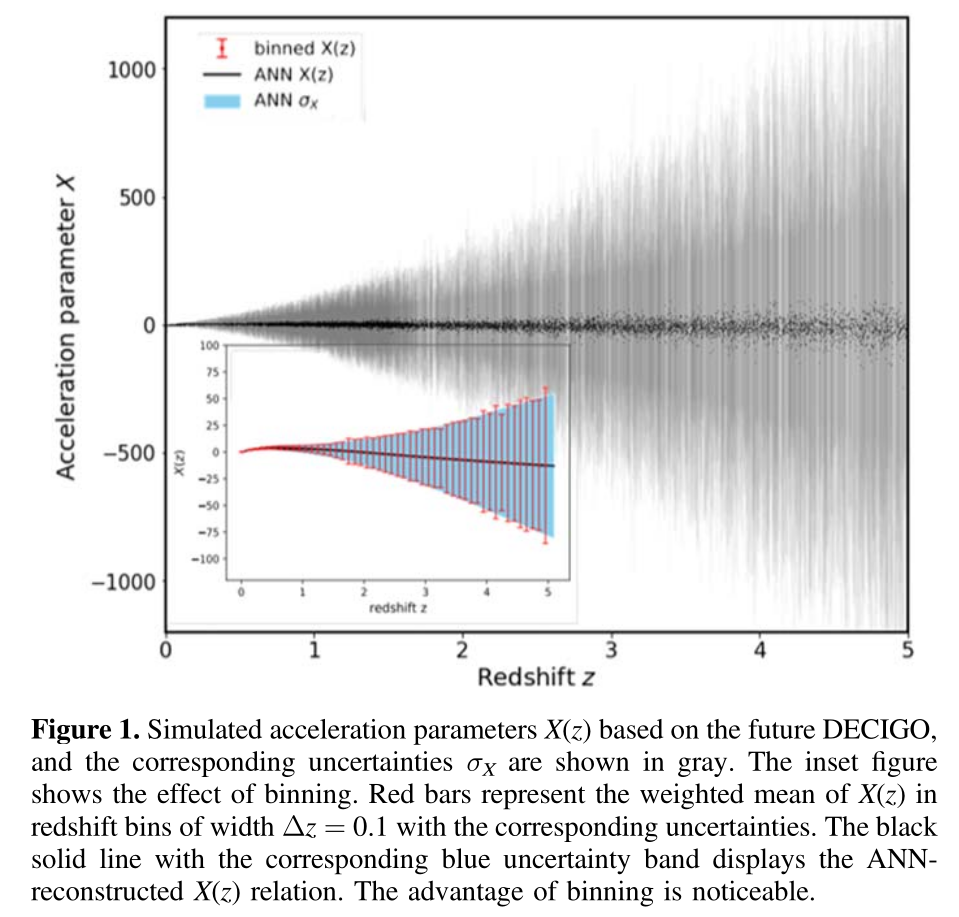
divide sample into 50 bins, train the ANN on the simulated $X(z)$ data and predicte the $X(z)$ at other redshifts.

ANN: input redshift $z$, output corresponding cosmic acceleration parameter $X(z)$ and its respective uncertainty $\sigma_X$ at that redshift.

Simulate data

ANN: input redshift $z$, output corresponding cosmic acceleration parameter $X(z)$ and its respective uncertainty $\sigma_X$ at that redshift.

QSOs $\rightarrow$ $D_{A}^{\text{obs}}(z)$

The characteristic angular size of a distant radio quasar is $$ \theta=\frac{2\sqrt{-\ln\Gamma\ln 2}}{\pi B} $$ $B$: the interferometer baseline
$\Gamma=S_c/S_t$: the ratio between the total and correlated flux densities The angular size of the compact structure in radio QSOs is

$$ \theta(z)=\frac{l_m}{D_A(z;\boldsymbol{p})} $$

$l_m$: the linear size scaling factor describing the apparent distribution of radio brightness within the core

$$ \theta(z)=\frac{l_m}{D_A(z;\boldsymbol{p})} $$

Taking $l_m=11.03\pm0.25\text{pc}$ and following the redshift distribution of QSOs from Palanque-Delabrouille et al.(2016)(https://doi.org/10.1051/0004-6361/201527392e),
simulate $1000$ "angular size-redshift" data, assume the "measured" angular sizes follow a Gaussian distribution $\theta_{\text{means}}=N(\theta_\text{fid},\sigma_\theta)$, $\theta_{\text{fid}}$ is obtained from equation above under same model in GW.

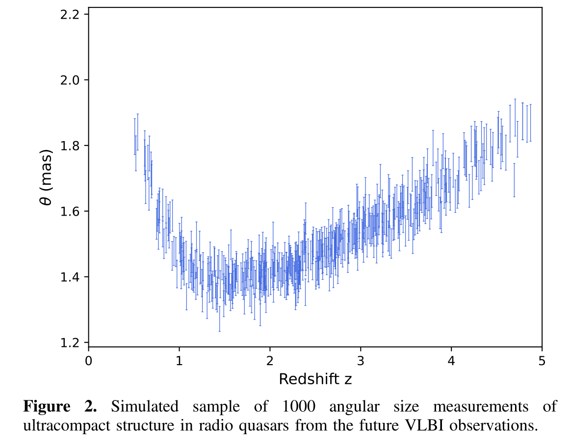
Taking $l_m=11.03\pm0.25\text{pc}$ and following the redshift distribution of QSOs from Palanque-Delabrouille et al.(2016)(https://doi.org/10.1051/0004-6361/201527392e),
simulate $1000$ "angular size-redshift" data, assume the "measured" angular sizes follow a Gaussian distribution $\theta_{\text{means}}=N(\theta_\text{fid},\sigma_\theta)$, $\theta_{\text{fid}}$ is obtained from equation above under same model in GW.

Results

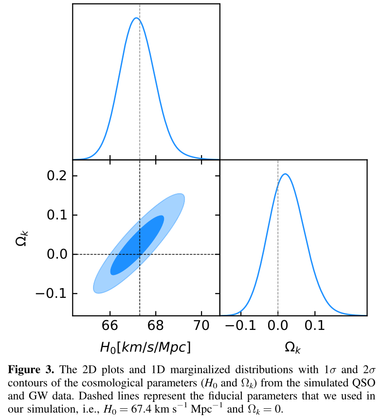
1. The best-fit values of $H_0$ and $\Omega_k$

using the Markov Chain Monte Carlo method to minimize the $\chi^2$ objective function: $$ \chi^2=\sum_{i=1}^{1000} \frac{[D_{A,i}^{\text{th}}(z;\boldsymbol{p})-D_{A,i}^{\text{obs}}(z)]^2}{\sigma_{D_{A,i}^{\text{th}}}^2+\sigma_{D_{A,i}^{\text{obs}}}^2} $$

here GW $\rightarrow$ $X(z)$ $\rightarrow$ $D_{A,i}^{\text{th}}(z;\boldsymbol{p})$
QSOs $\rightarrow$ $D_{A,i}^{\text{obs}}(z)$

1. The best-fit values of $H_0$ and $\Omega_k$

using the Markov Chain Monte Carlo method to minimize the $\chi^2$ objective function: $$ \chi^2=\sum_{i=1}^{1000} \frac{[D_{A,i}^{\text{th}}(z;\boldsymbol{p})-D_{A,i}^{\text{obs}}(z)]^2}{\sigma_{D_{A,i}^{\text{th}}}^2+\sigma_{D_{A,i}^{\text{obs}}}^2} $$

1. The best-fit values of $H_0$ and $\Omega_k$

$$ H_0=67.19_{-0.74}^{+0.77}\ \text{km}\ \text{s}^{-1}\ \text{Mpc}^{-1},\quad \Omega_k=0.022_{-0.046}^{+0.051} $$ at $68.3\%$ confidence level.

1. The best-fit values of $H_0$ and $\Omega_k$

$$ H_0=67.19_{-0.74}^{+0.77}\ \text{km}\ \text{s}^{-1}\ \text{Mpc}^{-1},\quad \Omega_k=0.022_{-0.046}^{+0.051} $$ at $68.3\%$ confidence level.

compare to used model $H_0=67.4\ \text{km}\ \text{s}^{-1}\ \text{Mpc}^{-1}$ and $\Omega_k=0$

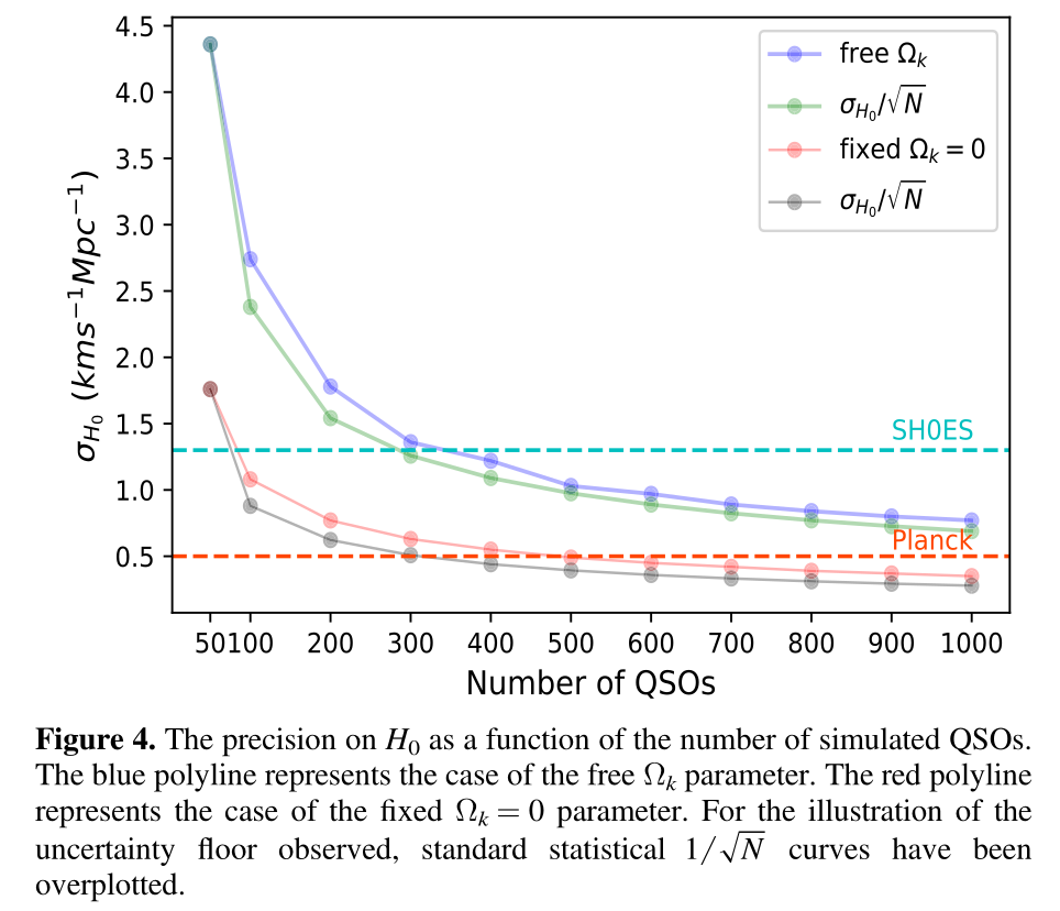
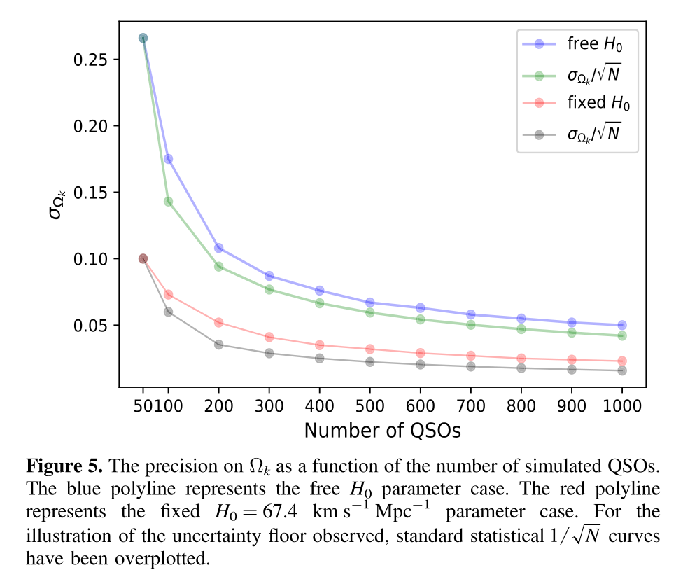
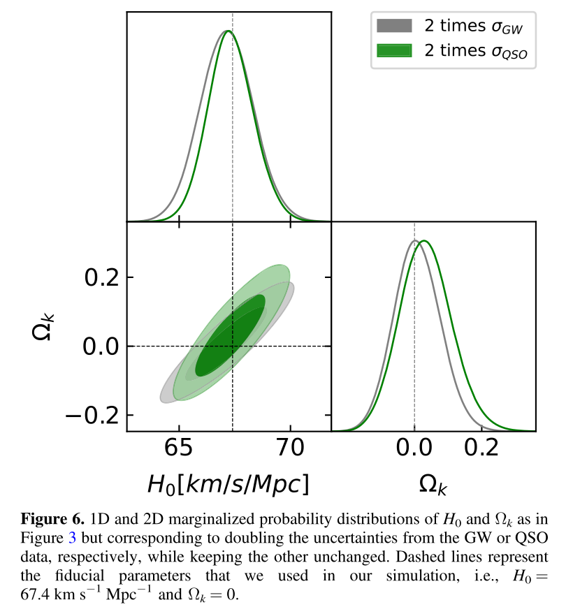
2. The uncertainties of the best-fit parameters as a function of QSO sample size $N$

3. The uncertainties related to GW signals and QSOs

Conclusion

Conclusion

1. a cosmological model-independent method to determine the Hubble constant and curvature parameter simultaneously based on GW from DECIGO and QSOs from VLBI

DECIGO $\rightarrow$ GW $\rightarrow$ phase shift $\rightarrow$ $H(z)$ $\rightarrow$ $D_{A,i}^{\text{th}}(z;\boldsymbol{p})$

VLBI $\rightarrow$ QSOs $\rightarrow$ "angular size-distance" $\rightarrow$ $D_{A,i}^{\text{obs}}(z)$

2. assume a fiducial cosmology to simulate GW and QSOs datas:

$N=1000$ QSOs $\rightarrow$ $\sigma_{H_0}=0.75\ \text{km}\ \text{s}^{-1}\ \text{Mpc}^{-1}$ and $\sigma_{\Omega_k}=0.048$ achieve $1\%$ precision

the precision of $H_0$ with a fixed prior on $\Omega_k$ can reach $0.5\%$

the performance of the method on QSO samples of different sizes (from $N=50$ to $N=1000$): not a simple $1/\sqrt{N}$ but saturate at $N=500$ (unsolved)

3. potential ways to improve results:

higher angular resolution and lower statistical and systematic uncertainty from QSOs from VLBI

datas from other astronomical probes such SNe Ia and BAOs

Thanks