Introduction to Perturbation Techniques

Nayfeh, A. H. (1993). Introduction to perturbation techniques. Wiley.

pdf with notes

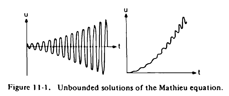
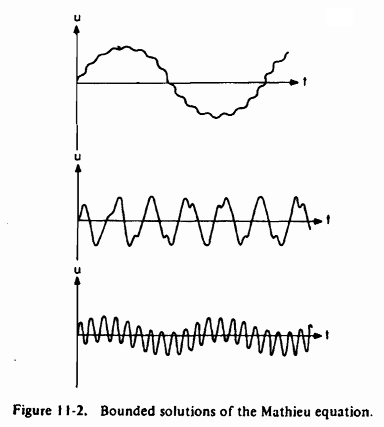
The Floquet theory to solve the Mathieu equation.
The detuning analysis used in forced oscillations.

9 Forced Oscillations

$$\ddot{u}+u+2\epsilon\mu\dot{u}+\epsilon u^3=F\cos\omega t \tag{9.4}$$

Resonances

$$u(t;\epsilon)=u_0(t)+\epsilon u_1(t)+\cdots \tag{9.5}$$

$$u=a\cos(t+\beta)+\frac{F}{1-\omega^2}\cos\omega t+\epsilon\left[\cdots+\frac{\cdots}{P(\omega)}+\cdots\right] \tag{9.16}$$

• primary or main resonance: $\omega\approx 1$
• secondary resonance: $\omega\approx 0,\dfrac{1}{3},3$

Detuning Analysis

Secondary Resonances

In this case $\omega$ is away from $1$.

If $\omega$ is away from $0$,

$$D_0^2 u+2\epsilon D_0D_1u+2\epsilon\mu D_0u+\cdots+u+\epsilon u^3=F\cos\omega T_0 \tag{9.19}$$

$$u=u_0(T_0,T_1)+\epsilon u_1(T_0,T_1)+\cdots,\quad T_1=\epsilon T_0$$

$$\begin{align} \mathrm{O}(\epsilon^0)\qquad\qquad & D_0^2u_0+u_0=F\cos\omega T_0 \tag{9.21} \\ \mathrm{O}(\epsilon^1)\qquad\qquad & D_0^2u_1+u_1=-2D_0D_1u_0-2\mu D_0u_0-u_0^3 \tag{9.22} \end{align}$$

for $\mathrm{O}(\epsilon^0)$

$$\begin{align} u_0&=a(T_1)\cos[T_0+\beta(T_1)]+2\Lambda\cos\omega T_0 \tag{9.23} \\ &=A(T_1)e^{iT_0}+\Lambda e^{i\omega T_0}+c.c. \tag{9.24} \end{align}$$

where

$$A=\frac{1}{2}ae^{i\beta},\quad \Lambda=\frac{F}{2(1-\omega^2)} \tag{9.25}$$

$u_0\rightarrow\mathrm{O}(\epsilon)$:

$$\begin{align} D_0^2u_1+u_1=&-[2i(A'+\mu A)+3(A\bar{A}+2\Lambda^2)A]e^{iT_0}-(2i\mu\omega+6A\bar{A}+3\Lambda^2)\Lambda e^{i\omega T_0} \\ &-A^3e^{3iT_0}-\Lambda^3 e^{3i\omega T_0}-3A^2\Lambda e^{i(2+\omega)T_0}-3\bar{A}^2\Lambda e^{i(\omega-2)T_0}-3A\Lambda^2 e^{i(1+2\omega)T_0} \\ &-3A\Lambda^2 e^{i(1-2\omega)T_0}+c.c. \end{align} \tag{9.26}$$

---

The Case $\omega\approx 3$

Introduce a detuning parameter $\sigma=\mathrm{O}(1)$ defined by

$$\omega=3+\epsilon\sigma$$

The secular terms in Eq.(9.26) are $e^{iT_0}$ and $e^{i(\omega-2)T_0}=e^{iT_0}e^{i\sigma T_1}$ (which generate secular term $T_0e^{iT_0}/2i$)

The solvability condition gives

$$2iA'+2i\mu A+3A^2\bar{A}+6A\Lambda^2+3\bar{A}^2\Lambda e^{i\sigma T_1}=0 \tag{9.30}$$

using Eq.(9.25), separate into read and imaginary parts

$$\begin{align} a'&=-\mu a-\dfrac{3}{4}a^2\Lambda \sin(\sigma T_1-3\beta) \tag{9.34} \\ a\beta'&=3a\Lambda^2+\dfrac{3}{8}a^3+\dfrac{3}{4}a^2\Lambda\cos(\sigma T_1-3\beta) \tag{9.35} \end{align}$$

this is a nonautonomous system with $T_1$ appears explicitly, transforming this into an autonomous system by introducing the new dependent variable $\gamma$ defined by

$$\gamma=\sigma T_1-3\beta \tag{9.37}$$

so we have the solution

$$u=a\cos\left(\frac{1}{3}\omega t-\frac{1}{3}\gamma\right)+2\Lambda\cos\omega t+\mathrm{O}(\epsilon) \tag{9.41}$$

$$\begin{align} a'&=-\mu a-\frac{3}{4}a^2\Lambda\sin\gamma \tag{9.39} \\ a\gamma'&=\sigma a-9a\Lambda^2-\frac{9}{8}a^3-\frac{9}{4}a^2\Lambda\cos\gamma \tag{9.40} \end{align}$$

---

The Case $\omega\approx\dfrac{1}{3}$

$$3\omega=1+\epsilon\sigma \tag{9.47}$$

$$D_0^2u_1+u_1=-[2iA'+2i\mu A+6\Lambda^2 A+3A^2\bar{A}]e^{iT_0}-\Lambda^3 e^{i\sigma T_1}e^{iT_0}+c.c.+\text{NST} \tag{9.49}$$

Similar process as above, finally gives solution

$$u=a\cos(2\omega t-\gamma)+2\Lambda\cos\omega t+\mathrm{O}(\epsilon) \tag{9.60}$$

$$\begin{align} a'&=-\mu a-\Lambda^3\sin\gamma \tag{9.57} \\ a\gamma'&=\sigma a-3\Lambda^2 a-\frac{3}{8}a^3-\Lambda^3\cos\gamma \tag{9.58} \end{align}$$

---

The Case $\omega\approx 0$

$$\omega=\epsilon\sigma$$

$$D_0^2 u+2\epsilon D_0D_1u+2\epsilon\mu D_0u+\cdots+u+\epsilon u^3=F\cos\sigma T_1 \tag{9.64}$$

$$\begin{align} \mathrm{O}(\epsilon^0)\qquad\qquad & D_0^2u_0+u_0=F\cos\sigma T_1 \tag{9.65} \\ \mathrm{O}(\epsilon^1)\qquad\qquad & D_0^2u_1+u_1=-2D_0D_1u_0-2\mu D_0u_0-u_0^3 \tag{9.66} \end{align}$$

for $\mathrm{O}(\epsilon^0)$ (homogeneous + particular)

$$u_0=Ae^{iT_0}+\bar{A}e^{-iT_0}+F\cos\sigma T_1 \tag{9.67}$$

$u_0\rightarrow\mathrm{O}(\epsilon)$:

$$D_0^2u_1+u_1=-2i(A'+\mu A)e^{iT_0}-3A^2\bar{A}e^{iT_0}-3F^2\cos^2\sigma T_1 Ae^{iT_0}+c.c.+\text{NST} \tag{9.68}$$

solvability condition gives

$$\begin{align} a'&=-\mu a \tag{9.71} \\ a\beta'&=\frac{3}{8}a^3+\frac{3}{2}F^2a\cos^2\sigma T_1 \tag{9.72} \end{align}$$

the exact solution is

$$a=a_0 e^{-\mu T_1} \tag{9.73}$$

$$\beta=-\frac{3}{16\mu}a_0^2 e^{-2\mu T_1}+\frac{3}{4}F^2T_1+\frac{3F^2}{8\sigma}\sin 2\sigma T_1+\beta_0 \tag{9.75}$$

$$\begin{align} u=&\ a_0e^{-\epsilon\mu t}\cos\left[\left(1+\frac{3}{4}\epsilon F^2\right)t-\frac{3}{16\mu}a_0^2e^{-2\epsilon\mu t}+\frac{3\epsilon F^2}{8\omega}\sin 2\omega t+\beta_0\right] \\ &+F\cos\omega t+\mathrm{O}(\epsilon) \end{align} \tag{9.77}$$

Primary Resonance

In this case $\omega\approx 1$

$u_0$ becomes very large as $\omega\rightarrow 1$, and the ordering of the terms above is rendered invalid.

Attempt 1: reorder the nonlinear $\epsilon u^3$ and the damping $2\epsilon\mu\dot{u}$ terms to appear at $\mathrm{O}(\epsilon^0)$, thereby balancing the effect of the primary-resonance excitation. However, this choice leads to the original equation at $\mathrm{O}(\epsilon^0)$.

Attempt 2: reorder the excitation $F\cos\omega t$ so that it appears at $\mathrm{O}(\epsilon)$ where the nonlinear and damping terms first appear. Let $F=\epsilon f$

$$\ddot{u}+u+2\epsilon\mu\dot{u}+\epsilon u^3=\epsilon f\cos\omega t \tag{9.82}$$

$$\begin{align} \mathrm{O}(\epsilon^0)\qquad\qquad & D_0^2u_0+u_0=0 \tag{9.84} \\ \mathrm{O}(\epsilon^1)\qquad\qquad & D_0^2u_1+u_1=-2D_0D_1u_0-2\mu D_0u_0-u_0^3+f\cos\omega T_0 \tag{9.86} \end{align}$$

for $\mathrm{O}(\epsilon^0)$

$$u_0=A(T_1)e^{iT_0}+\bar{A}(T_1)e^{-iT_0} \tag{9.87}$$

$u_0\rightarrow\mathrm{O}(\epsilon)$:

$$D_0^2u_1+u_1=-(2iA'+2i\mu A+3A^2\bar{A})e^{iT_0}-A^3e^{3iT_0}+\frac{1}{2}f e^{i\omega T_0}+c.c. \tag{9.88}$$

Introduce detuning parameter $\sigma$ defined by

$$\omega=1+\epsilon\sigma \tag{9.89}$$

$$D_0^2u_1+u_1=-(2iA'+2i\mu A+3A^2\bar{A})e^{iT_0}+\frac{1}{2}fe^{i\sigma T_1}e^{iT_0}+c.c.+\text{NST} \tag{9.91}$$

then follow the process in the case $\omega\approx 3,\frac{1}{3}$ to obtain the exact solution

$$u=a\cos(\omega t-\gamma)+\mathrm{O}(\epsilon) \tag{9.100}$$

$$\begin{align} a'&=-\mu a+\frac{1}{2}f\sin\gamma \tag{9.98} \\ a\gamma'&=\sigma a-\frac{3}{8}a^3+\frac{1}{2}f\cos\gamma \tag{9.99} \end{align}$$

11 The Mathieu Equation

$$\ddot{u}+(\delta+2\epsilon\cos 2t)u=0 \tag{11.2}$$

The Floquet Theory

(11.2) is a second-order linear homogeneous equation, it possesses two linearly independent solutions $u_1(t)$ and $u_2(t)$ satisfying the initial conditions

$$\begin{array}{cc} u_1(0)=1 & \dot{u}_1(0)=0 \\ u_2(0)=0 & \dot{u}_2(0)=1 \end{array}\tag{11.13}$$

The solutions have a period of $\pi$, the evolution equation in matrix notation is

$$\boldsymbol{u}(t+\pi)=\boldsymbol{A}\boldsymbol{u}(t) \tag{11.20}$$

$$\boldsymbol{A}=\left[\begin{array}{cc} u_1(\pi) & \dot{u}_1(\pi) \\ u_2(\pi) & \dot{u}_2(\pi) \end{array}\right]\quad \boldsymbol{u}=\left[\begin{array}{c} u_1 \\ u_2 \end{array}\right] \tag{11.21}$$

Try diagonalizing the matrix $\boldsymbol{A}$, we have a diagonal matrix $\boldsymbol{B}$ whose eigenvalues are given by

$$\lambda^2-\text{tr}(\boldsymbol{A})\lambda+1=0 \tag{11.32}$$

$$\lambda_{1,2}=\frac{\text{tr}(\boldsymbol{A})\pm\sqrt{[\text{tr}(\boldsymbol{A})]^2-4}}{2} \tag{11.34}$$

And the evolution equation gives

$$\boldsymbol{v}(t+\pi)=\boldsymbol{B}\boldsymbol{v}(t) \tag{11.27}$$

$$\boldsymbol{B}=\boldsymbol{P}\boldsymbol{A}\boldsymbol{P}^{-1} \tag{11.29}$$

$$\boldsymbol{u}(t)=\boldsymbol{P}^{-1}\boldsymbol{v}(t) \tag{11.24}$$

---

(a) When the diagonal matrix has the form

$$\boldsymbol{B}=\left[\begin{array}{cc} \lambda_1 & 0 \\ 0 & \lambda_2 \end{array}\right] \tag{11.35}$$

The evolution equation reads,

$$\begin{array}{c} \boldsymbol{v}_1(t+\pi)=\lambda_1\boldsymbol{v}_1(t) \\ \boldsymbol{v}_2(t+\pi)=\lambda_2\boldsymbol{v}_2(t) \end{array} \tag{11.38}$$

$$\boldsymbol{v}_1(t+n\pi)=\lambda_1^n\boldsymbol{v}_1(t) \tag{11.39}$$

So $\lambda_1=\lambda_2=\pm 1$ separate stable from unstable solutions and are usually referred to as transition values.

Solving Eq.(11.38) which named normal or Floquet form

$$e^{-\gamma_1(t+\pi)}v_1(t+\pi)=\lambda_1e^{-\gamma_1\pi}e^{-\gamma_1 t}v_1(t) \tag{11.43}$$

The exact solution is

$$\boldsymbol{v}_{1,2}(t)=e^{\gamma_{1,2} t}\phi_{1,2}(t) \tag{11.46,11.48}$$

where $\phi_{1,2}(t)$ is arbitrary function satisfing $\phi_{1,2}(t+\pi)=\phi_{1,2}(t)$, and the characteristic exponent is

$$\gamma_{1,2}=\frac{1}{\pi}\ln \lambda_{1,2} \tag{11.44}$$

---

(b) When $\boldsymbol{A}$ is not diagonalizable, the matrix $\boldsymbol{B}$ has the form

$$\boldsymbol{B}=\left[\begin{array}{cc} 1 & 0 \\ 1 & 1 \end{array}\right] \text{ or }\left[\begin{array}{cc} -1 & 0 \\ 1 & -1 \end{array}\right]\equiv\left[\begin{array}{cc} \lambda & 0 \\ 1 & \lambda \end{array}\right] \tag{11.37}$$

The normal / Floquet form

$$\begin{align} v_1(t+\pi)&=\lambda v_1(t) \tag{11.49a} \\ v_2(t+\pi)&=\lambda v_2(t)+v_1(t) \tag{11.49b} \end{align}$$

The solution for $v_1(t)$ is the same as (a)

$$\begin{array}{c} \boldsymbol{v}_1(t)=e^{\gamma t}\phi_1(t) \\ \phi_1(t+\pi)=\phi_1(t) \quad\text{and}\quad \gamma=\dfrac{1}{\pi}\ln \lambda \end{array} \tag{11.50}$$

for $v_2(t)$,

$$e^{-\gamma(t+\pi)}v_2(t+\pi)=e^{-\gamma t}v_2(t)+\frac{1}{\lambda}\phi_1(t) \tag{11.51}$$

$$\boldsymbol{v}_2(t)=e^{\gamma t}[\phi_2(t)+\frac{t}{\pi\lambda}\phi_1(t)],\ \phi_2(t+\pi)=\phi_2(t) \tag{11.52}$$

---

$$\lambda_{1,2}=\frac{\text{tr}(\boldsymbol{A})\pm\sqrt{[\text{tr}(\boldsymbol{A})]^2-4}}{2} \tag{11.34}$$

When $|\text{tr}(\boldsymbol{A})|>2$, the solutions contains one unbounded and another bounded with time.

When $|\text{tr}(\boldsymbol{A})|<2$, the solutions are bounded.