天文数据处理

时间序列处理

插值

对于时间间隔 $Δ t$ 不均匀的离散时间序列，可以通过插值补充为时间间隔固定的序列。

使用 python 中 scipy 模块里的 interpolate.interp1d 进行插值：

interpolate.interp1d(x, y, kind='linear')

参数 `kind`	插值方法
`linear`	线性插值
`nearest`,`nearest_up`	最邻近阶梯插值
`zero`	零阶样条插值
`slinear`	一阶样条插值
`quadratic`	二阶样条插值
`cubic`	三阶样条插值
`previous`,`next`	阶梯插值

对应 matlab 中的 interp1(t, y, t_uniform, kind)

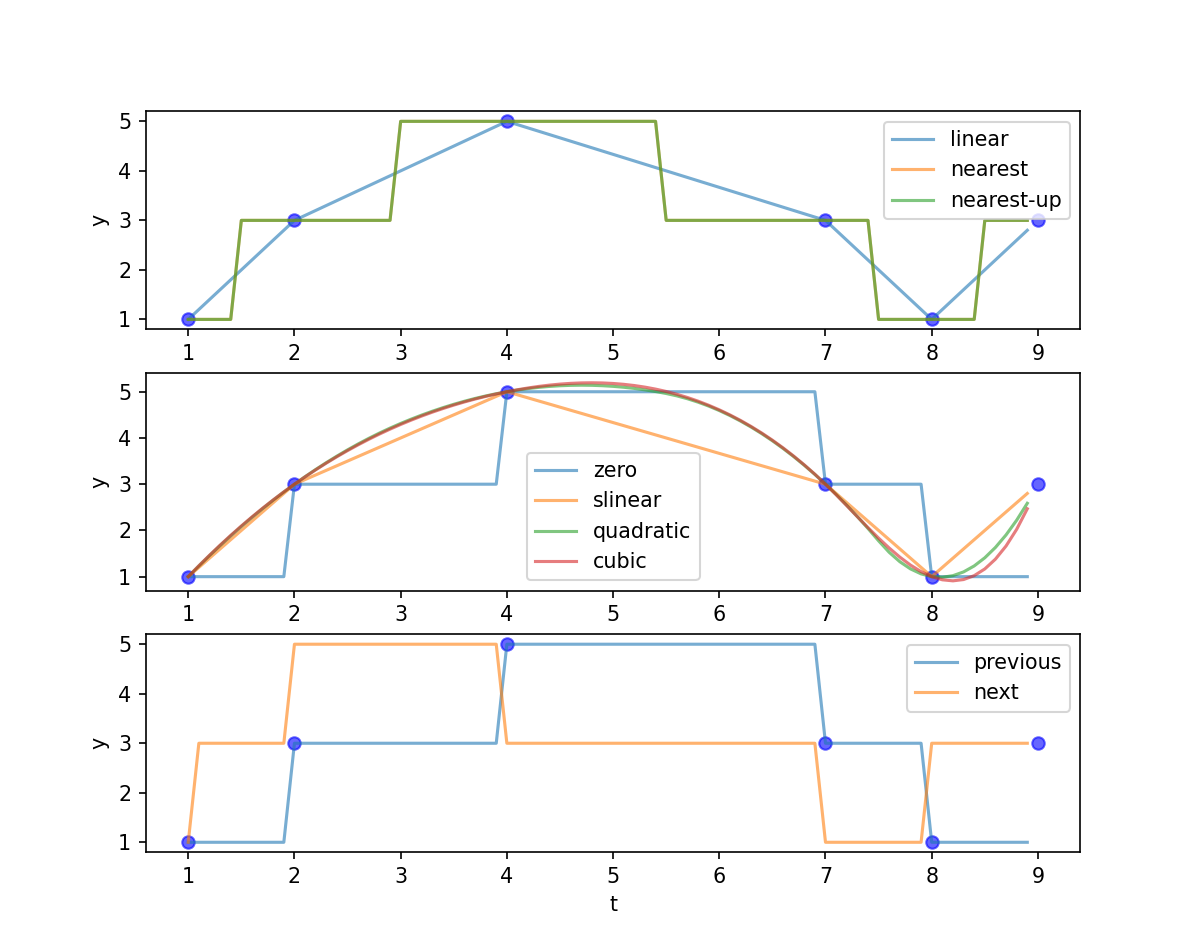
脚本

pymatlab

import numpy as np
import matplotlib.pyplot as plt
from scipy import interpolate

t = np.array([1, 2, 4, 7, 8, 9])
y = np.array([1, 3, 5, 3, 1, 3])

t_new = np.arange(1, 9, 0.1)
kinds = ['linear', 'nearest', 'nearest-up',
         'zero', 'slinear', 'quadratic', 'cubic',
         'previous', 'next']

ax1 = plt.subplot(311)
ax2 = plt.subplot(312)
ax3 = plt.subplot(313)

ax1.scatter(t, y, c='b', alpha=0.6)
for kind in kinds[:3]:
    func = interpolate.interp1d(t, y, kind=kind)
    y_new = func(t_new)
    ax1.plot(t_new, y_new, label=kind, alpha=0.6)
ax1.set_xlabel('t')
ax1.set_ylabel('y')
ax1.legend()

ax2.scatter(t, y, c='b', alpha=0.6)
for kind in kinds[3:-2]:
    func = interpolate.interp1d(t, y, kind=kind)
    y_new = func(t_new)
    ax2.plot(t_new, y_new, label=kind, alpha=0.6)
ax2.set_xlabel('t')
ax2.set_ylabel('y')
ax2.legend()

ax3.scatter(t, y, c='b', alpha=0.6)
for kind in kinds[-2:]:
    func = interpolate.interp1d(t, y, kind=kind)
    y_new = func(t_new)
    ax3.plot(t_new, y_new, label=kind, alpha=0.6)
ax3.set_xlabel('t')
ax3.set_ylabel('y')
ax3.legend()

plt.show()

matlab

t = [1, 2, 4, 7, 8, 9];
y = [1, 3, 5, 3, 1, 3];

t_new = 1:0.1:9;
kinds = {'linear', 'nearest', 'next', 'previous', 'pchip', 'spline', 'makima', 'nearest', 'next'};

subplot(3,1,1);
scatter(t, y, 36, 'b', 'filled', 'MarkerFaceAlpha', 0.6); hold on;
for i = 1:3
    y_new = interp1(t, y, t_new, kinds{i});
    plot(t_new, y_new, 'DisplayName', kinds{i}, 'LineWidth', 1.2, 'LineStyle', '-');
end
legend;

subplot(3,1,2);
scatter(t, y, 36, 'b', 'filled', 'MarkerFaceAlpha', 0.6); hold on;
for i = 4:6
    y_new = interp1(t, y, t_new, kinds{i});
    plot(t_new, y_new, 'DisplayName', kinds{i}, 'LineWidth', 1.2, 'LineStyle', '-');
end
legend;

subplot(3,1,3);
scatter(t, y, 36, 'b', 'filled', 'MarkerFaceAlpha', 0.6); hold on;
for i = 7:8
    y_new = interp1(t, y, t_new, kinds{i});
    plot(t_new, y_new, 'DisplayName', kinds{i}, 'LineWidth', 1.2, 'LineStyle', '-');
end
legend;

hold off;

平滑处理

理论

常用的时间序列的平滑模型有：

滑动平均模型
加权滑动平均模型
二次滑动平均模型
指数平滑模型

滑动平均模型

$n$ 阶滑动平均即以每 $n$ 个连续数据的平均值代替该区域中点处的数据

x^{'} (t_{j}) = \frac{1}{n} \sum_{i = j - δ}^{j + δ} x (t_{i}), j = δ + 1, δ + 2, . . ., N - δ

（ $n$ 为奇数，记 $δ = \frac{n + 1}{2}$ ）

加权滑动平均模型

在滑动平均模型中加入权重 $α_{i}$

x^{'} (t_{j}) = \frac{1}{n} \sum_{i = j - δ}^{j + δ} α_{i} x (t_{i}), j = δ + 1, δ + 2, . . ., N - δ

（其中加权因子满足 $\frac{1}{n} \sum_{i} α_{i} = 1$ ）

二次滑动平均模型

对经过一次滑动平均的序列再进行一次滑动平均。

指数平滑模型

4-1. 简单指数平滑法

S_{t} = A y_{t} + (1 - A) S_{t - 1}

4-2. 线性指数平滑法

S_{t} = A y_{t} + (1 - A) (S_{t - 1} + b_{t - 1})

加入趋势效应

b_{t} = B (S_{t} - S_{t - 1}) + (1 - B) b_{t - 1}

实践

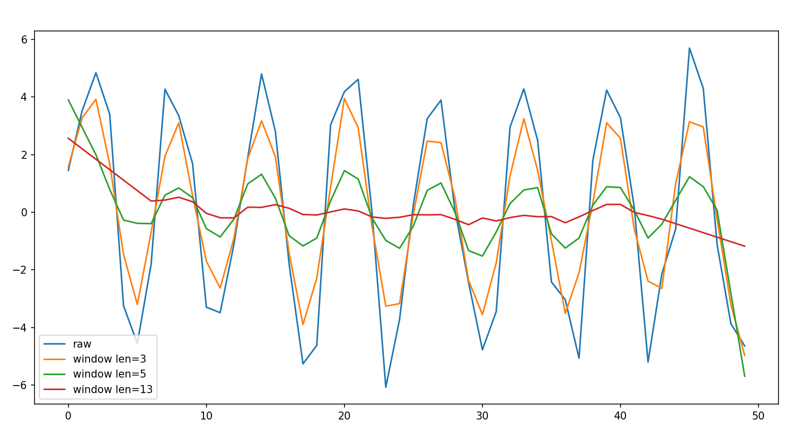
使用 python 中 scipy 模块里的 signal.savgol_filter 进行平滑：

signal.savgol_filter(x, window_length, polyorder)

取 polyorder=1 ，该函数会对数据 x 进行 window_length 阶滑动平均。

python 脚本

import numpy as np
import matplotlib.pyplot as plt
from scipy import signal

t = np.arange(0, 50, 1)
x = 5 * np.sin(t)
noise = np.random.randn(50)
y = x + noise

window_lens = [3, 5, 13]

plt.plot(y, label='raw')
for l in window_lens:
    y_new = signal.savgol_filter(y, l, 1)
    plt.plot(y_new, label=f'window len={l}')
plt.legend()
plt.show()

曲线拟合

理论

最小二乘法

拟合函数模型 $f (t_{i}) = a_{0} + a_{1} t_{i} + a_{2} t_{i}^{2} + . . . + a_{m} t_{i}^{m}$

取参数使残差平方和 $Δ = \sum_{i = 1}^{n} [y (t_{i}) - f (t_{i})]^{2}$ 最小

即

\frac{\partial Δ}{\partial a_{i}} = \frac{\partial}{\partial a_{j}} \sum_{i = 1}^{n} [y (t_{i}) - f (t_{i})]^{2} = 0, j = 0, 1, . . ., m

实例：参考作业2

矩阵法

对数据 $x_{i} = [0.1, 0.4, 0.5, 0.7, 0.7, 0.9], y_{i} = [0.61, 0.92, 0.99, 1.52, 1.47, 2.03]$ 做线性回归

有超定线性方程

a_{1} x_{i} + a_{0} = y_{i}, i = 1, 2, . . ., 6

写成矩阵形式

X A = Y

其中

X = [\begin{array}{cc} 0.1 & 1 \\ 0.4 & 1 \\ 0.5 & 1 \\ 0.7 & 1 \\ 0.7 & 1 \\ 0.9 & 1 \end{array}], A = [\begin{matrix} a_{1} \\ a_{0} \end{matrix}], Y = [\begin{matrix} 0.61 \\ 0.92 \\ 0.99 \\ 1.52 \\ 1.47 \\ 2.03 \end{matrix}]

等式两边同时左乘矩阵 $X^{T}$

X^{T} X A = X^{T} Y \Rightarrow A = (X^{T} X)^{- 1} X^{T} Y

验证程序

import numpy as np
import matplotlib.pyplot as plt

xi = np.array([0.1, 0.4, 0.5, 0.7, 0.7, 0.9])
yi = np.array([0.61, 0.92, 0.99, 1.52, 1.47, 2.03])

# using polyfit
an = np.polyfit(xi, yi, 1)
p = np.poly1d(an)
print('polyfit:', p)

# using matrix
cons = np.ones(6)
X = np.c_[xi, cons]
X_t = X.T
X_tX_inv = np.linalg.inv(X_t@X)
A = X_tX_inv@X_t@yi
print('manual:', f'{A[0]}x+{A[1]}')

x_fit = np.arange(0, 1, 0.01)
y_fit1 = p(x_fit)
y_fit2 = A[0]*x_fit + A[1]

plt.scatter(xi, yi, label='raw data')
plt.plot(x_fit, y_fit1, 'r-.', alpha=0.6, label='polyfit fit')
plt.plot(x_fit, y_fit2, 'g:', alpha=0.6, label='manual fit')
plt.legend()
plt.show()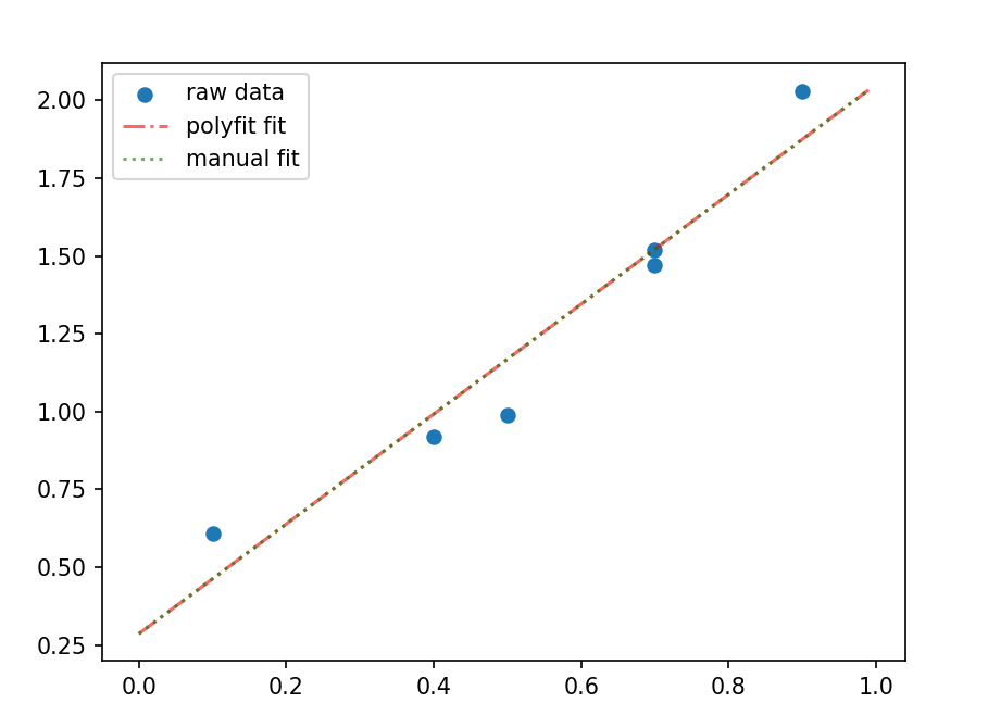

实践

使用 python 中 scipy 模块里 optimize.curve_fit 进行拟合：

optimize.curve_fit(f, xdata, ydata)

自行编写函数模型 f(x, params) ，将待拟合的数据 xdata,ydata 传入函数后会返回参数数组和协方差。

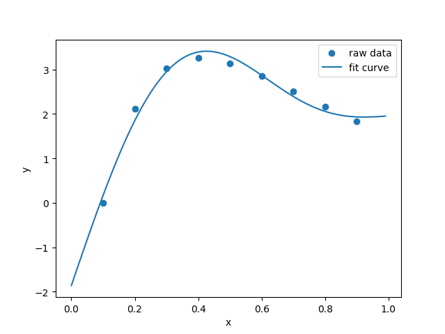
实例：

使用曲线模型 $g (x) = c_{1} + c_{2} x + c_{3} \sin (π x) + c_{4} \sin (2 π x)$ 对下面数据进行拟合：

$x_{i} = [0.1, 0.2, 0.3, 0.4, 0.5, 0.6, 0.7, 0.8, 0.9]$

$y_{i} = [0, 2.122, 3.0244, 3.2568, 3.1399, 2.8579, 2.514, 2.1639, 1.8358]$

python 脚本

import numpy as np
import matplotlib.pyplot as plt
from scipy.optimize import curve_fit

# raw data
xi = np.array([0.1, 0.2, 0.3, 0.4, 0.5,
               0.6, 0.7, 0.8, 0.9])
yi = np.array([0, 2.122, 3.0244, 3.2568, 3.1399,
               2.8579, 2.514, 2.1639, 1.8358])

# use g(x)=c1+c2x+c3sin(pi*x)+c4sin(2pi*x) to fit
def func(x, c1, c2, c3, c4):
    return c1 + c2*x + c3*np.sin(np.pi*x) + c4*np.sin(2*np.pi*x)

popt, pcov = curve_fit(func, xi, yi)
x_fit = np.arange(0, 1, 0.01)
y_fit = func(x_fit, popt[0], popt[1], popt[2], popt[3])

# draw
plt.scatter(xi, yi, label='raw data')
plt.plot(x_fit, y_fit, label='fit curve')
plt.xlabel('x')
plt.ylabel('y')
plt.legend()
plt.show()

时域频域转换

傅里叶变换

理论

查看傅里叶变换

实践

使用 python 中 scipy 模块里的 fftpack.fft 进行傅里叶变换：

fftpack.fft(x, N)

但是该函数只是返回数据进行傅里叶变换后的复数序列，还需要转化成频谱图。

def FFT(data, T):
    L = len(data)
    N = int(np.power(2, np.ceil(np.log2(L))))
    FFT_y = np.abs(fft(data, N)) / L * 2
    Fre = np.arange(int(N/2)) * L / N / T
    FFT_y = FFT_y[range(int(N/2))]
    return Fre, FFT_y

实例：

绘制如下两个周期信号的频谱图

T = 2
fs = 5000
f1 = 404
f2 = 2000
f3 = 1234

t = np.linspace(0, T, T*fs)

base = 2
component1 = 2*np.sin(2*np.pi*f1*t)
component2 = 5*np.sin(2*np.pi*f2*t+1)
component3 = 3*np.sin(2*np.pi*f3*t+4)
noise = np.random.normal(1, 10, T*fs)
y1 = base+component1+component2+component3
y2 = component1+component2+component3+noise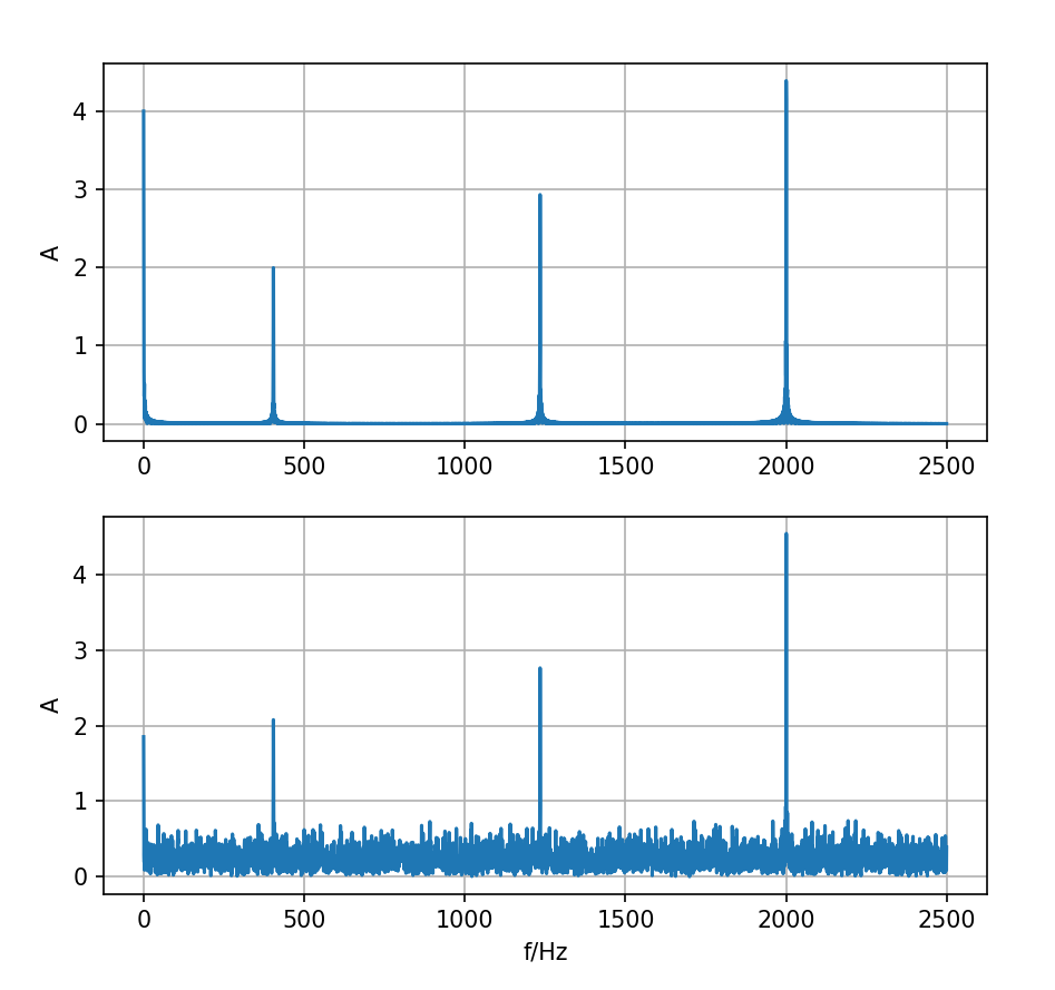

python 脚本

import numpy as np
import matplotlib.pyplot as plt
from scipy.fftpack import fft

def FFT(data, T):
    L = len(data)
    N = int(np.power(2, np.ceil(np.log2(L))))
    FFT_y = np.abs(fft(data, N)) / L * 2
    Fre = np.arange(int(N/2)) * L / N / T
    FFT_y = FFT_y[range(int(N/2))]
    return Fre, FFT_y

T = 2
fs = 5000
f1 = 404
f2 = 2000
f3 = 1234

t = np.linspace(0, T, T*fs)

base = 2
component1 = 2*np.sin(2*np.pi*f1*t)
component2 = 5*np.sin(2*np.pi*f2*t+1)
component3 = 3*np.sin(2*np.pi*f3*t+4)
noise = np.random.normal(1, 10, T*fs)
y1 = base+component1+component2+component3
y2 = component1+component2+component3+noise

ax1 = plt.subplot(211)
ax2 = plt.subplot(212)
fre1, fft_y1 = FFT(y1, T)
fre2, fft_y2 = FFT(y2, T)
ax1.plot(fre1, fft_y1)
ax2.plot(fre2, fft_y2)
ax1.set_ylabel('A')
ax1.grid()
ax2.set_ylabel('A')
ax2.set_xlabel('f/Hz')
ax2.grid()
plt.show()

上面绘图结果 $2000 H z$ 处的振幅比 $5$ 小，是由于快速傅里叶变化时补充到 2 的幂次项数据较多。可以将采样时长 T 改为 3 秒，这样得到的结果更好。

matlab 脚本

matlab

T = 2;
fs = 5000;
f1 = 404;
f2 = 2000;
f3 = 1234;

t = linspace(0, T, fs*T);

base = 2;
component1 = 2*sin(2*pi*f1*t);
component2 = 5*sin(2*pi*f2*t+1);
component3 = 3*sin(2*pi*f3*t+4);
noise = randn(1, fs*T);
y1 = base + component1 + component2 + component3;
y2 = component1 + component2 + component3 + noise;

% fft
ffty1 = fft(y1);
ffty1_abs = abs(ffty1) * 2 / length(y1);
fre1 = (0:length(y1)-1)*fs/length(y1);
ffty2 = fft(y2);
ffty2_abs = abs(ffty2) * 2 / length(y2);
fre2 = (0:length(y2)-1)*fs/length(y2);

% plot
figure;
ax1 = subplot(2, 1, 1);
ax2 = subplot(2, 1, 2);
plot(ax1, fre1, ffty1_abs);
plot(ax2, fre2, ffty2_abs);

逆傅里叶变换

理论

把信号 ${f_{j}}$ 经过 FFT 得到的复数序列 ${c_{k}}$ 通过 IFFT 变回信号 ${f_{j}}$

实践

使用 scipy.fftpack.ifft 进行逆傅里叶变换：

fftpack.ifft(x, N)

实例：

pythonmatlab

python

import numpy as np
import matplotlib.pyplot as plt
from scipy.fftpack import fft, ifft

# generate signal
T = 2
fs = 100
L = T * fs
t = np.linspace(0, T, L)
signal = 5 + 3 * np.cos(2 * np.pi * 7 * t) + 2 * np.sin(2 * np.pi * 10 * t)

# use fftpack.fft to fft
N = int(np.power(2, np.ceil(np.log2(L))))
fft_y = fft(signal, N)
fft_y_abs = 2 * np.abs(fft_y) / L
fre = np.arange(int(N/2)) * L / (N * T)
fft_y_abs = fft_y_abs[:int(N/2)]

# use fftpack.ifft to rebuild signal
signal_rebuild = ifft(fft_y, N)
signal_rebuild = signal_rebuild[:L]

# draw result
ax1 = plt.subplot(211)
ax2 = plt.subplot(212)
ax1.plot(fre, fft_y_abs)
ax1.set_xlabel('f/Hz')
ax1.set_ylabel('A')
ax2.plot(t, signal, label='raw signal')
ax2.plot(t, signal_rebuild, 'r--', label='rebuild signal', alpha=0.7)
ax2.set_xlabel('t/s')
ax2.set_ylabel('signal')
ax2.legend()
plt.show()

matlab

% generate signal
T = 2;
fs = 100;
L = T * fs;
t = linspace(0, T, L);
signal = 5 + 3 * cos(2 * pi * 7 * t) + 2 * sin(2 * pi * 10 * t);

% fft
fft_y = fft(signal);
fft_y_abs = abs(fft_y) * 2 / L;
fre = (0:L-1) / T;

% ifft
signal_rebuild = ifft(fft_y);

% plot
figure;
subplot(2, 1, 1);
plot(fre, fft_y_abs);
xlabel('f/Hz');
ylabel('A');
subplot(2, 1, 2);
plot(t, signal, 'DisplayName', 'raw signal');
hold on;
plot(t, signal_rebuild, 'r--', 'DisplayName', 'rebuild signal');
xlabel('t/s');
ylabel('signal');
legend('show');
hold off;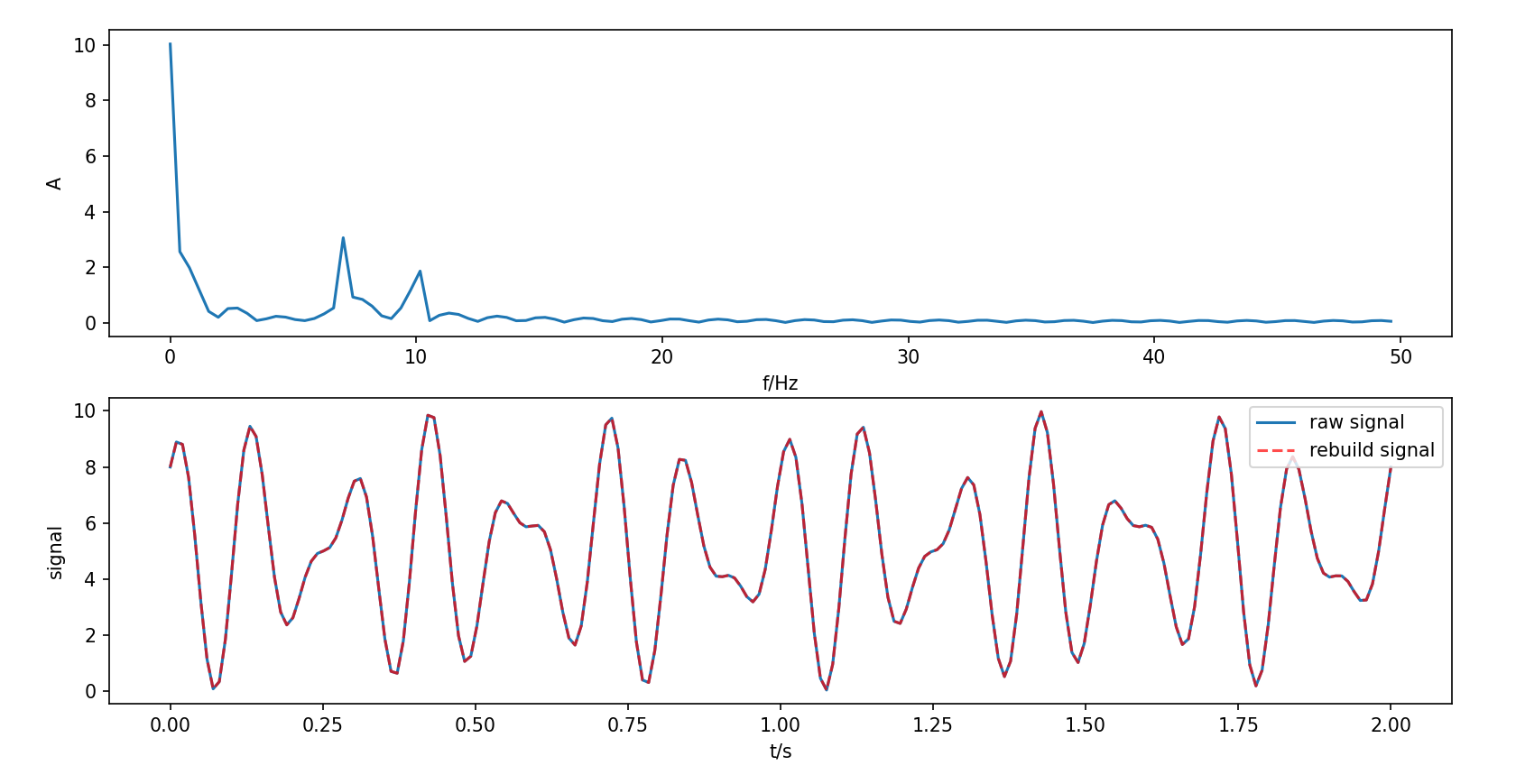

滤波

理论

对原信号 FFT 变换后的复数序列中想要去除的频率部分改为 0 再逆傅里叶变换即可。

实践

实例：把上一节使用的信号中 $10 H z$ 部分滤掉。

pythonmatlab

python

import numpy as np
import matplotlib.pyplot as plt
from scipy.fftpack import fft, ifft

# generate signal
T = 2
fs = 100
L = T * fs
t = np.linspace(0, T, L)
signal = 5 + 3 * np.cos(2 * np.pi * 7 * t) + 2 * np.sin(2 * np.pi * 10 * t)
signal_rm10 = 5 + 3 * np.cos(2 * np.pi * 7 * t)

# use fftpack.fft to fft
N = int(np.power(2, np.ceil(np.log2(L))))
fft_y = fft(signal, N)
fre = np.arange(N) * L / (N * T)

# filtering on fft_y
# remove f between 9 Hz and 11 Hz
fre_remove = np.array([9, 11]) * N * T / L
fre_rm_1, fre_rm_2 = int(fre_remove[0]), int(fre_remove[1])+1
fre_rm_3, fre_rm_4 = N - fre_rm_2, N - fre_rm_1
fft_y[fre_rm_1:fre_rm_2] = 0
fft_y[fre_rm_3:fre_rm_4] = 0

# the fft_y after filtering
fft_y_abs = 2 * np.abs(fft_y) / L

# use fftpack.ifft to rebuild signal
signal_filtering = ifft(fft_y, N)
signal_filtering = signal_filtering[:L]

# draw result
ax1 = plt.subplot(211)
ax2 = plt.subplot(212)
ax1.plot(fre, fft_y_abs)
ax1.set_xlabel('f/Hz')
ax1.set_ylabel('A')
ax2.plot(t, signal_rm10, label='raw signal remove 10Hz part')
ax2.plot(t, signal_filtering, 'r--', label='signal after filtering', alpha=0.7)
ax2.set_xlabel('t/s')
ax2.set_ylabel('signal')
ax2.legend()
plt.show()

matlab

% generate signal
T = 2;
fs = 100;
L = T * fs;
t = linspace(0, T, L);
signal = 5 + 3 * cos(2 * pi * 7 * t) + 2 * sin(2 * pi * 10 * t);
signal_rm10 = 5 + 3 * cos(2 * pi * 7 * t);

% fft
fft_y = fft(signal);
fre = (0:L-1) / T;

% filtering
fre_remove = [9, 11] * T + 1;
fre_rm_1 = floor(fre_remove(1));
fre_rm_2 = ceil(fre_remove(2));
fre_rm_3 = L - fre_rm_2;
fre_rm_4 = L - fre_rm_1;
fft_y(fre_rm_1:fre_rm_2) = 0;
fft_y(fre_rm_3:fre_rm_4) = 0;
fft_y_abs = abs(fft_y) * 2 / L;

% ifft
signal_filtering = ifft(fft_y);

% plot
figure;
subplot(2, 1, 1);
plot(fre, fft_y_abs);
xlabel('f/Hz');
ylabel('A');
subplot(2, 1, 2);
plot(t, signal_rm10, 'DisplayName', 'raw signal remove 10Hz part');
hold on;
plot(t, signal_filtering, 'r--', 'DisplayName', 'signal after filtering');
xlabel('t/s');
ylabel('signal');
legend('show');
hold off;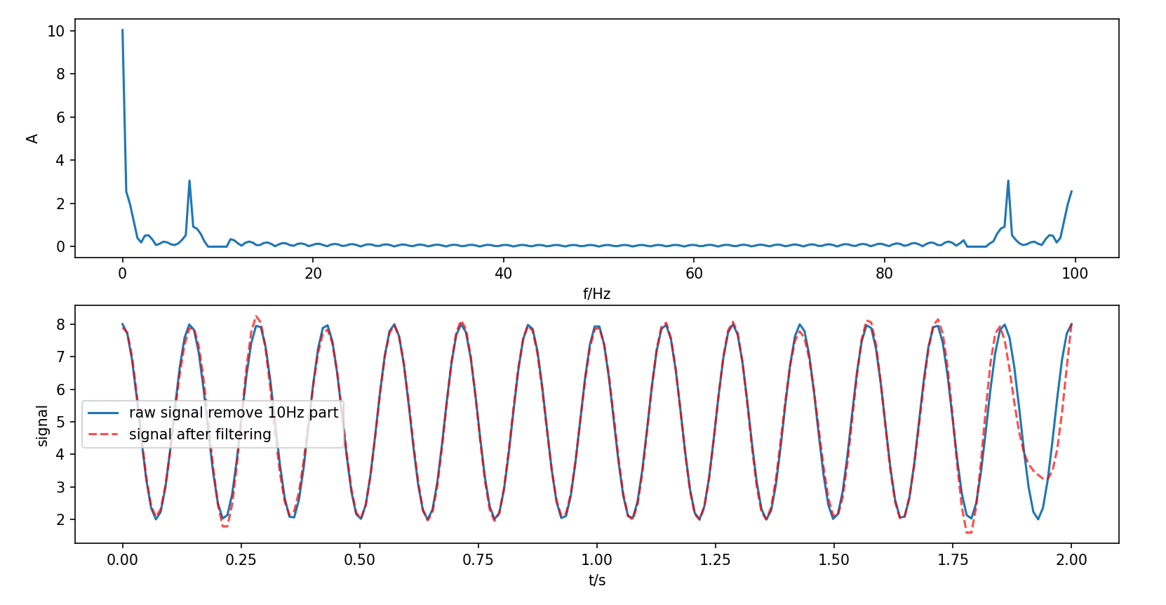

谱分析的数字化问题

采样定理

采样定理（奈奎斯特-香农采样定理）：为了不失真地把连续时间信号转成离散时间信号，并在后续过程能够完全恢复原信号，需要满足采样频率至少是信号中最高频率的两倍。

f_{s} \geq 2 f_{m a x}

奈奎斯特频率 $f_{N} = \frac{f_{s}}{2}$ ，任何高于 $f_{N}$ 的信号成分将无法被正确采样，导致混叠。

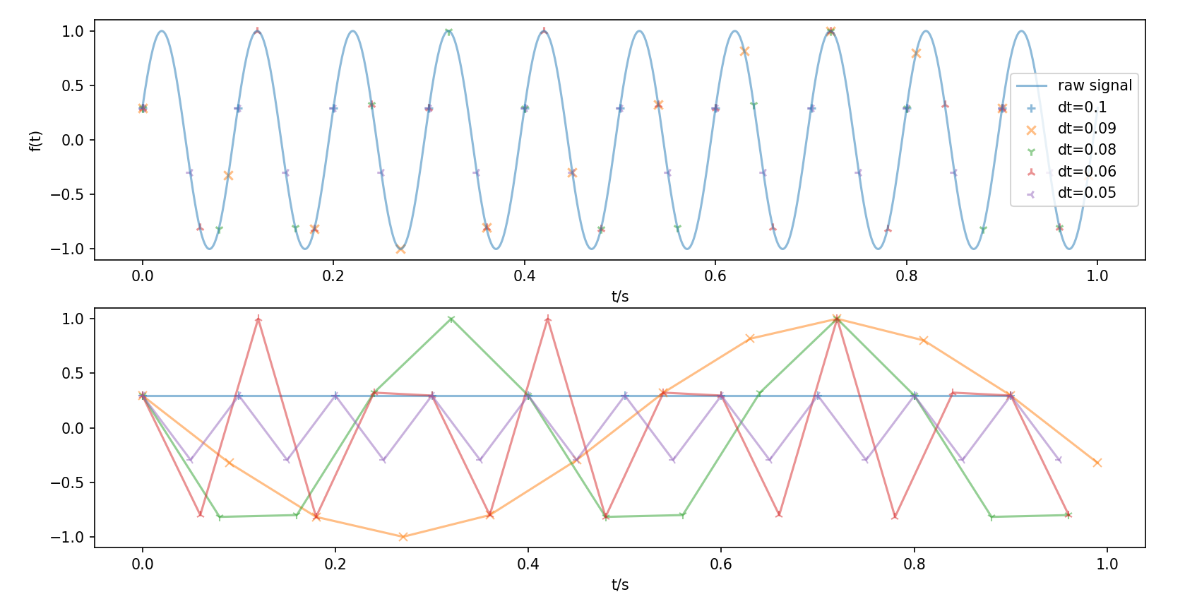
python脚本

import numpy as np
import matplotlib.pyplot as plt

def f(x):
    f0 = 10
    return np.sin(2 * np.pi * f0 * x + 0.3)

t0 = np.arange(0, 1.001, 0.001)
y = f(t0)

dts = [0.1, 0.09, 0.08, 0.06, 0.05]
markers = ['+', 'x', '1', '2', '3']

ax1 = plt.subplot(211)
ax2 = plt.subplot(212)
ax1.plot(t0, y, label='raw signal', alpha=0.5)
ax1.set_xlabel('t/s')
ax1.set_ylabel('f(t)')
for i in range(5):
    dt = dts[i]
    ts = np.arange(0, 1, dt)
    ys = f(ts)
    ax1.scatter(ts, ys, label=f'dt={dt}', alpha=0.5, marker=markers[i])
    ax2.plot(ts, ys, label=f'dt={dt}', alpha=0.5, marker=markers[i])
ax1.legend()
ax2.set_xlabel('t/s')
plt.show()

频谱泄露和窗函数

频谱泄露

由于原信号是无限长的，而采集信号为有限长，在进行 FFT 时，这种截断会导致频谱泄露。

e.g.

例如对于无限长正弦信号 $\sin (2 π \cdot 9 t)$ ，我们进行 $2 s, 100 H z$ 的采样，然后进行傅里叶变换得到频谱图：

import numpy as np
import matplotlib.pyplot as plt
from scipy.fftpack import fft

T = 2
fs = 100
L = T * fs
t = np.linspace(0, T, L)
signal = np.sin(2 * np.pi * 9 * t)

fft_y = fft(signal)
fft_y_abs = 2 * np.abs(fft_y) / L
fre = np.arange(L) / T

plt.plot(fre, fft_y_abs)
plt.show()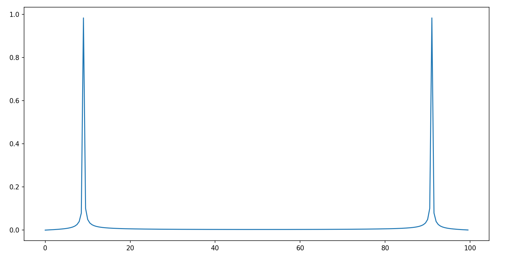

可以发现除了主瓣（ $9 H z$ ）外，其他频率振幅很小但不为零。

窗函数

窗函数是一个有限长的函数，用于乘以原始信号的截断部分。

定义：窗函数 $w (t)$ 在区间 $[- T / 2, T / 2]$ 内变化，满足：

归一化 $\int_{- T / 2}^{T / 2} w (t) d t = 1$
非负性 $w (t) \geq 0$

作用：

减少频谱泄露
改善频谱分辨率（控制主瓣宽度）

常用的窗函数：

矩形窗

w (t) = {\begin{cases} \frac{1}{T} & | t | \leq \frac{T}{2} \\ 0 & | t | > \frac{T}{2} \end{cases}

主瓣最窄：矩形窗的主瓣宽度最小，对单个频率的分辨率最高。

旁瓣最高：矩形窗的旁瓣是最高的，导致频谱泄漏最严重。

汉宁窗(hanning)

w (t) = \frac{1}{T} \cos^{2} (\frac{π}{T} t)

主瓣较宽：主瓣宽度是矩形窗的两倍。

旁瓣较低：旁瓣高度显著降低。

哈明窗(hamming)

w (t) = \frac{1}{T} (0.54 + 0.46 \cos \frac{2 π t}{T})

主瓣宽度与汉宁窗类似。

旁瓣更低：哈明窗的旁瓣低于汉宁窗。

布莱克曼窗(Blackman)

w (t) = 0.4209 - 0.5109 \cos \frac{2 π t}{T} + 0.0691 \cos \frac{4 π t}{T}

主瓣更宽。

旁瓣非常低：布莱克曼窗的旁瓣极低，泄漏最小。

凯赛窗(Kaiser)

w (t) = \frac{I_{0} (β \sqrt{1 - (\frac{t}{T})^{2}})}{I_{0} (β)}

其中 $I_{0}$ 是修正的 0 阶第一类 Bessel 函数， $β$ 是控制窗函数形状的参数。

旁瓣高度可以用过 $β$ 调节： $β$ 增大，旁瓣降低，主瓣变宽。

减小主瓣宽度和抑制旁瓣是一对矛盾，只能根据不同用途折中处理。下面演示了各种窗函数在时域和频域上的作用：

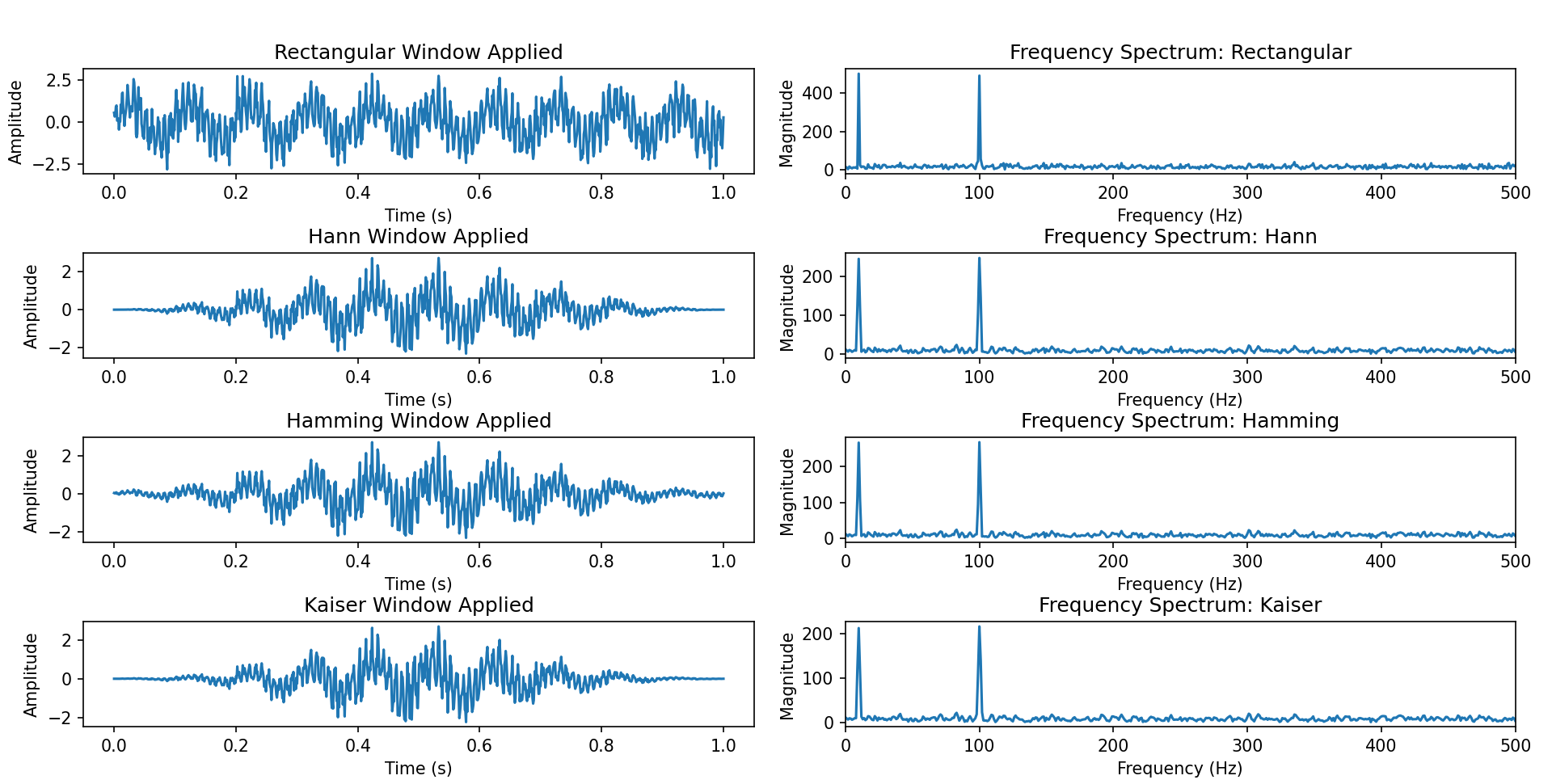
python脚本

import numpy as np
import matplotlib.pyplot as plt
from scipy.fftpack import fft

# 生成示例信号
fs = 1000  # 采样率
T = 1      # 信号总时长
f1 = 10    # 信号频率1
f2 = 100   # 信号频率2
noise_amplitude = 0.5  # 噪声幅度

t = np.linspace(0, T, int(fs * T))
x = np.sin(2 * np.pi * f1 * t) + np.sin(2 * np.pi * f2 * t)
x += noise_amplitude * np.random.randn(len(t))

def rectangular_window(N):
    """矩形窗"""
    return np.ones(N)

def hann_window(N):
    """汉宁窗"""
    return np.hanning(N)

def hamming_window(N):
    """哈明窗"""
    return np.hamming(N)

def kaiser_window(N, beta=8.0):
    """凯塞窗"""
    return np.kaiser(N, beta)

def compute_spectrum(x, window):
    """计算信号的频谱"""
    x_windowed = x * window
    X = fft(x_windowed)
    freq = np.arange(len(X)) / T
    return freq, np.abs(X)

window_names = ['Rectangular', 'Hann', 'Hamming', 'Kaiser']
windows = [
    rectangular_window(len(x)),
    hann_window(len(x)),
    hamming_window(len(x)),
    kaiser_window(len(x))
]

fig, axes = plt.subplots(len(windows), 2, figsize=(12, 8))
plt.suptitle("Frequency Spectrum with Different Windows", y=1.05)

for idx, (window, name) in enumerate(zip(windows, window_names)):
    axes[idx, 0].plot(t, x * window)
    axes[idx, 0].set_title(f"{name} Window Applied")
    axes[idx, 0].set_xlabel("Time (s)")
    axes[idx, 0].set_ylabel("Amplitude")

    freq, spectrum = compute_spectrum(x, window)
    axes[idx, 1].plot(freq, spectrum)
    axes[idx, 1].set_title(f"Frequency Spectrum: {name}")
    axes[idx, 1].set_xlabel("Frequency (Hz)")
    axes[idx, 1].set_ylabel("Magnitude")
    axes[idx, 1].set_xlim(0, fs / 2)

plt.tight_layout()
plt.show()

功率谱估计

定义

功率谱密度 (Power Spectral Density,PSD) 描述信号功率在频域的分布，是自相关函数的傅里叶变换（维纳-辛钦定理）

S (f) = F [R (τ)]

其中 $R (τ) = lim_{T \to \infty} [\frac{1}{T} \int_{- T / 2}^{T / 2} f (t) f (t - τ) d t]$ 是信号的自相关函数。

功率谱估计

周期图法 (Periodogram)

直接对信号进行傅里叶变换后平方并归一化，得到功率谱估计：

\hat{S} (f) = \frac{1}{N} {| \sum_{n = 0}^{N - 1} x (n) e^{- j 2 π f n} |}^{2}

pythonmatlab

python

import numpy as np
import matplotlib.pyplot as plt
from scipy.signal import periodogram

fs = 1000
t = np.arange(0, 1, 1/fs)
x = np.sin(2 * np.pi * 100 * t) + 0.5 * np.random.randn(len(t))

# 周期图法
f, Pxx = periodogram(x, fs)
plt.semilogy(f, Pxx)
plt.xlabel('Frequency [Hz]')
plt.ylabel('PSD [V²/Hz]')
plt.title('Periodogram')
plt.show()

matlab

fs = 1000;
t = 0:1/fs:1-1/fs; % 确保与 Python 的 np.arange(0, 1, 1/fs) 对齐
x = sin(2 * pi * 100 * t) + 0.5 * randn(1, length(t));

% 周期图法
n = length(x);
xdft = fft(x); % 计算 FFT
xdft = xdft(1:floor(n/2)+1); % 取一半频率
psdx = (1/(fs*n)) * abs(xdft).^2; % 计算功率谱密度
psdx(2:end-1) = 2*psdx(2:end-1); % 调整功率
f = 0:fs/length(x):fs/2; % 频率向量

% 绘制功率谱密度
semilogy(f, psdx);
xlabel('Frequency [Hz]');
ylabel('PSD [V^2/Hz]');
title('Periodogram');
grid on;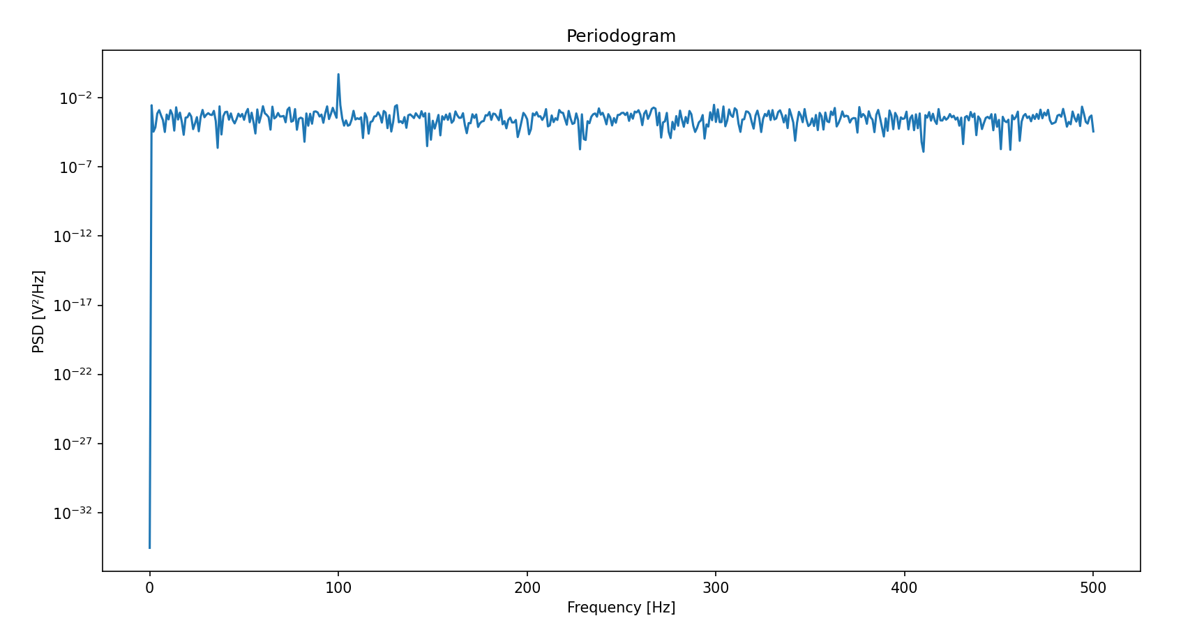

多段平均周期图法 (Bartlett)

将信号分为不重叠的K段，每段计算周期图后平均：

\hat{S} (f) = \frac{1}{K} \sum_{i = 1}^{K} {\hat{S}}_{i} (f)

pythonmatlab

python

import numpy as np
import matplotlib.pyplot as plt
from scipy.signal import periodogram

fs = 1000
t = np.arange(0, 1, 1/fs)
x = np.sin(2 * np.pi * 100 * t) + 0.5 * np.random.randn(len(t))

def bartlett_psd(x, fs, nperseg):
    K = len(x) // nperseg  # 分段数
    Pxx = 0
    for i in range(K):
        seg = x[i * nperseg : (i+1) * nperseg]
        f, Pxx_seg = periodogram(seg, fs)
        Pxx += Pxx_seg
    Pxx /= K
    return f, Pxx

# 多段平均周期图法
f, Pxx = bartlett_psd(x, fs, nperseg=256)
plt.semilogy(f, Pxx)
plt.xlabel('Frequency [Hz]')
plt.ylabel('PSD [V²/Hz]')
plt.title('Bartlett Method')
plt.show()

matlab

% MATLAB 实现 Bartlett 方法
fs = 1000;
t = 0:1/fs:1-1/fs; % 确保与 Python 的 np.arange(0, 1, 1/fs) 对齐
x = sin(2 * pi * 100 * t) + 0.5 * randn(1, length(t));

% Bartlett 方法实现
nperseg = 256; % 每段的长度
K = floor(length(x) / nperseg); % 分段数
Pxx = zeros(1, nperseg/2+1); % 初始化功率谱密度

for i = 1:K
    seg = x((i-1)*nperseg+1:i*nperseg); % 提取每段数据
    xdft = fft(seg); % 计算 FFT
    xdft = xdft(1:nperseg/2+1); % 取一半频率
    Pxx_seg = (1/(fs*nperseg)) * abs(xdft).^2; % 计算功率谱密度
    Pxx_seg(2:end-1) = 2*Pxx_seg(2:end-1); % 调整功率
    Pxx = Pxx + Pxx_seg; % 累加每段的功率谱密度
end
Pxx = Pxx / K; % 取平均值
f = 0:fs/nperseg:fs/2; % 频率向量

% 绘制功率谱密度
semilogy(f, Pxx);
xlabel('Frequency [Hz]');
ylabel('PSD [V^2/Hz]');
title('Bartlett Method');
grid on;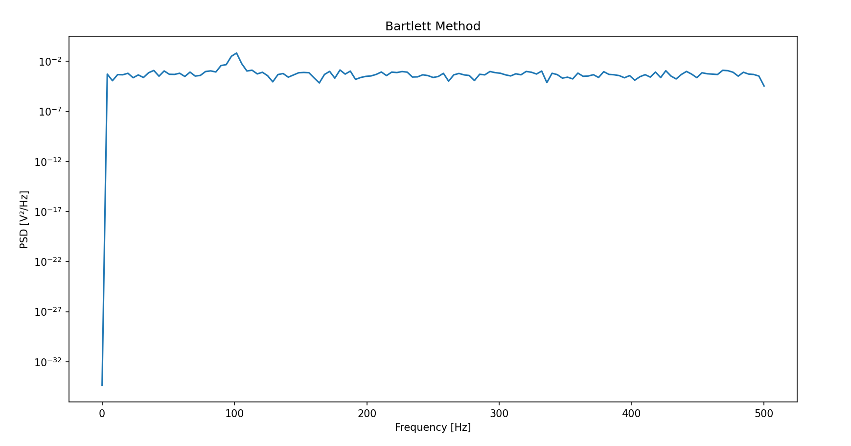

Welch 法

允许分段重叠并加窗，进一步减少方差和频谱泄漏：

\hat{S} (f) = \frac{1}{K U} \sum_{i = 1}^{K} | X_{i} (f) |^{2}

其中 $U$ 是窗函数的功率归一化因子。

pythonmatlab

python

import numpy as np
import matplotlib.pyplot as plt
from scipy.signal import welch

fs = 1000
t = np.arange(0, 1, 1/fs)
x = np.sin(2 * np.pi * 100 * t) + 0.5 * np.random.randn(len(t))

# Welch法（50%重叠，汉宁窗）
f, Pxx = welch(x, fs, nperseg=256, noverlap=128, window='hann')
plt.semilogy(f, Pxx)
plt.xlabel('Frequency [Hz]')
plt.ylabel('PSD [V²/Hz]')
plt.title('Welch Method')
plt.show()

matlab

% MATLAB 实现 Welch 方法
fs = 1000;
t = 0:1/fs:1-1/fs; % 确保与 Python 的 np.arange(0, 1, 1/fs) 对齐
x = sin(2 * pi * 100 * t) + 0.5 * randn(1, length(t));

% Welch 方法（50% 重叠，汉宁窗）
nperseg = 256; % 每段的长度
noverlap = 128; % 重叠部分的长度
window = hann(nperseg); % 汉宁窗

[Pxx, f] = pwelch(x, window, noverlap, nperseg, fs);

% 绘制功率谱密度
semilogy(f, Pxx);
xlabel('Frequency [Hz]');
ylabel('PSD [V^2/Hz]');
title('Welch Method');
grid on;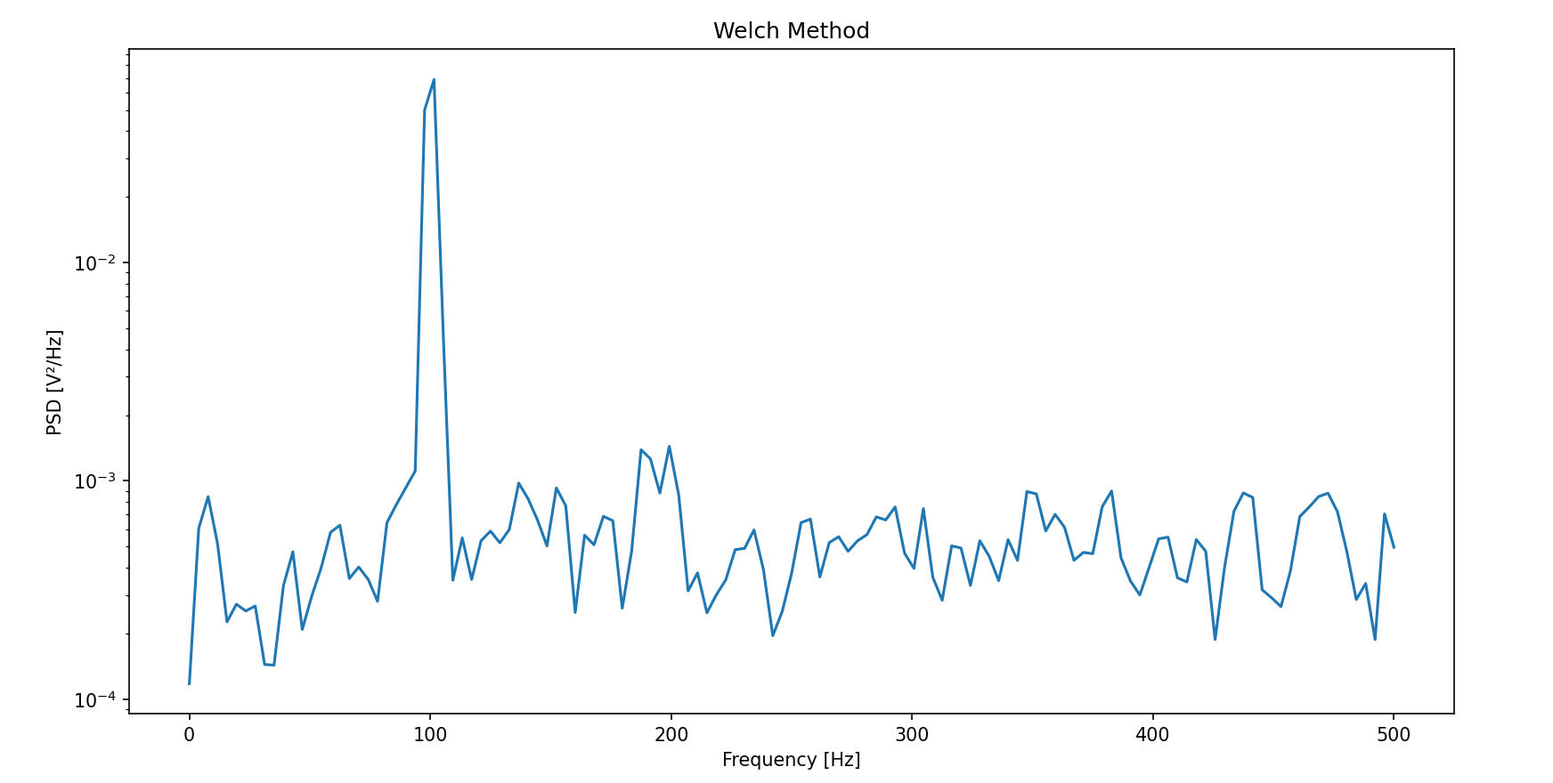

多窗口法 (Multitaper Method, MTM)

python:使用多个正交的Slepian窗口（DPSS序列）分别计算功率谱后平均，平衡方差和分辨率。

matlab:调用函数 pmtm(x, Nw, Nfft, fs)

pythonmatlab

python

import numpy as np
import matplotlib.pyplot as plt
from scipy.signal import windows, csd, periodogram

fs = 1000
t = np.arange(0, 1, 1/fs)
x = np.sin(2 * np.pi * 100 * t) + 0.5 * np.random.randn(len(t))

# 生成Slepian窗口
NW = 4  # 时间带宽积
Kmax = 2 * NW - 1  # 窗口数量
tapers = windows.dpss(len(x), NW, Kmax)

# 计算多窗口功率谱
Pxx = 0
for taper in tapers:
    f, Pxx_seg = periodogram(x * taper, fs)
    Pxx += Pxx_seg
Pxx /= len(tapers)

plt.semilogy(f, Pxx)
plt.xlabel('Frequency [Hz]')
plt.ylabel('PSD [V²/Hz]')
plt.title('Multitaper Method (MTM)')
plt.show()

matlab

fs = 1000;
t = 0:1/fs:1-1/fs; % 确保与 Python 的 np.arange(0, 1, 1/fs) 对齐
x = sin(2 * pi * 100 * t) + 0.5 * randn(1, length(t));
% multitaper method
[pxx, f] = pmtm(x, 4, 256, fs);
% plot
semilogy(f, pxx);
xlabel('Frequency [Hz]');
ylabel('PSD [V^2/Hz]');
title('Multitaper Method');
grid on;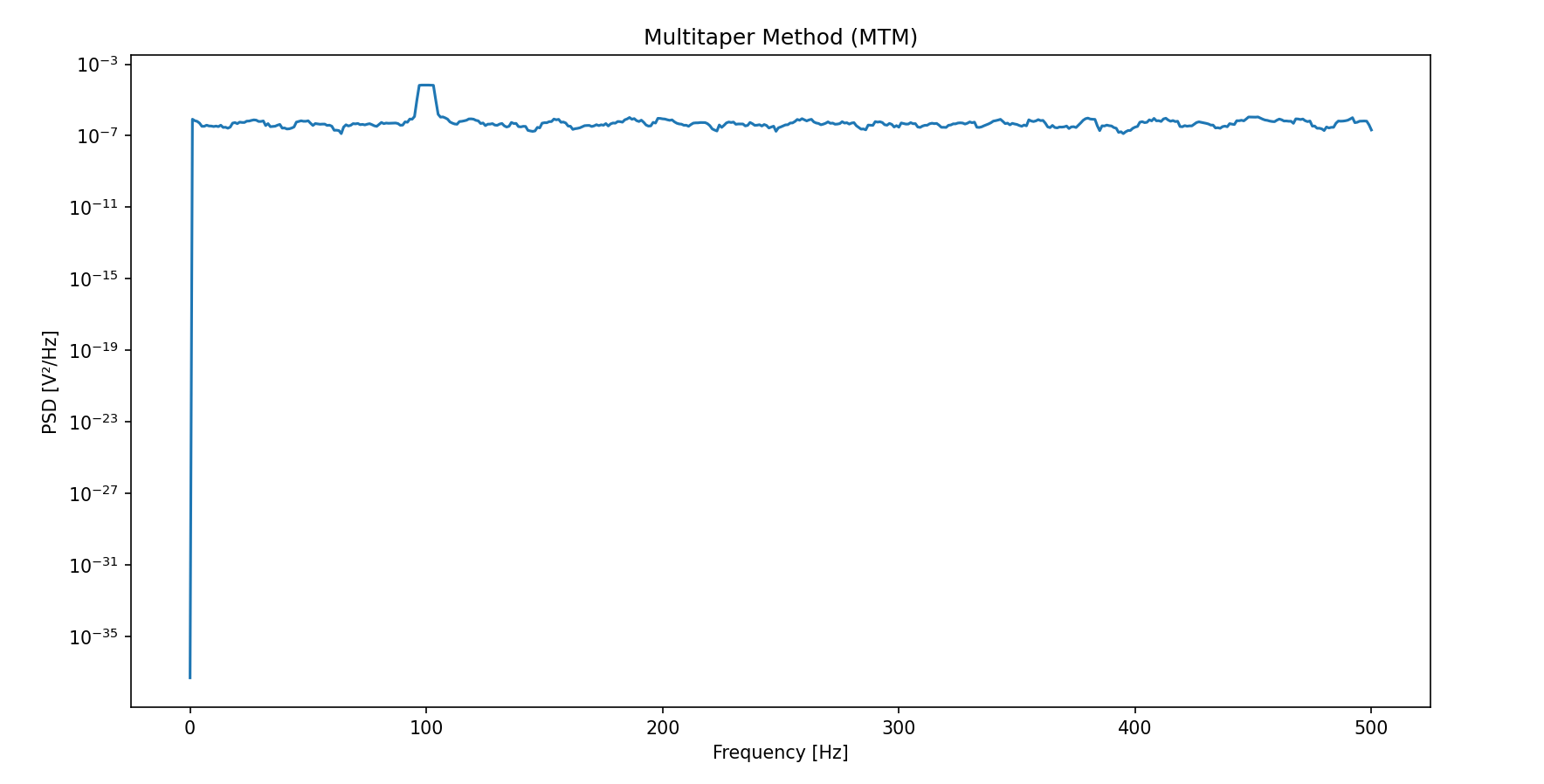

多信号分类法( MUSIC 法 )(Multiple Signal Classification)

调用matlab函数pmusic(x, [P, thresh], Nfft, fs, window, Noverlap)

matlab

fs = 1000; N = 1024; Nfft = 256; n = 0:N-1;
t = n/fs;
randn('state',0);
window = hanning(256);
xn = sin(2*pi*50*t) + 2*sin(2*pi*120*t) + randn(1,N);
[pxx, f] = pmusic(xn, [7, 1.1], Nfft, fs, window, 128);
plot(f, pxx);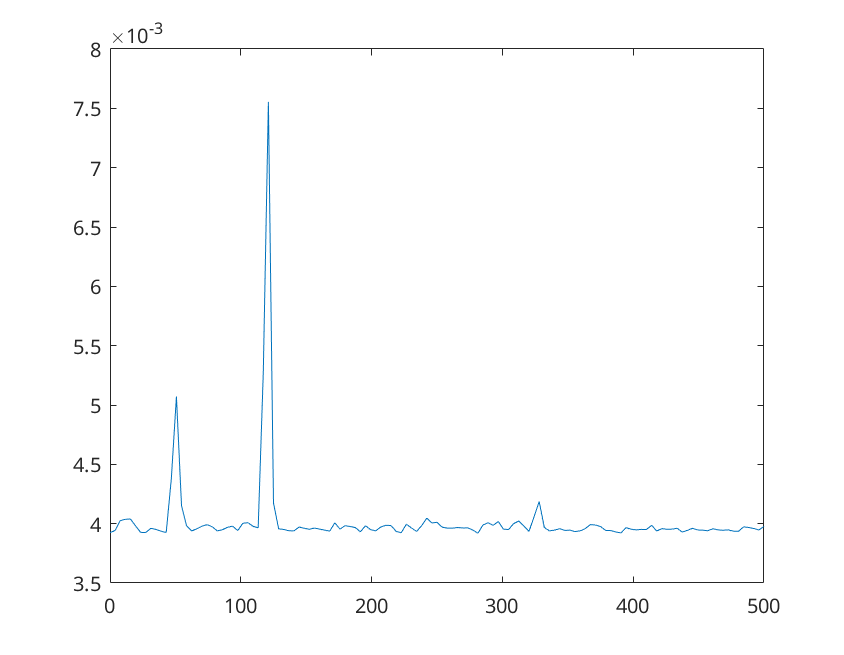

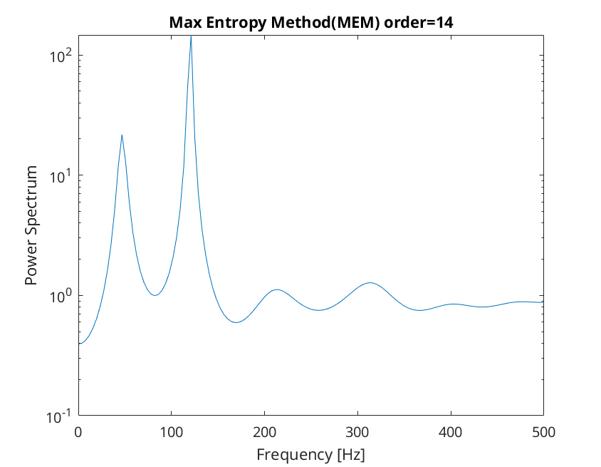
最大熵功率估计( MEM 法 )(Maximum Entropy Method)

调用matlab函数pmem(x, p, Nfft, fs)

matlab

fs = 1000; N = 1024; Nfft = 256; n = 0:N-1;
t = n/fs;
randn('state',0);
xn = sin(2*pi*50*t) + 2*sin(2*pi*120*t) + randn(1,N);
[pxx, f] = pmem(xn, 14, Nfft, fs);
semilogy(f, pxx);
xlabel('Frequency [Hz]');
ylabel('Power Spectrum');
title('Max Entropy Method(MEM) order=14');

天文数据处理 ​

时间序列处理 ​

插值 ​

平滑处理 ​

理论 ​

实践 ​

曲线拟合 ​

理论 ​

实践 ​

时域频域转换 ​

傅里叶变换 ​

理论 ​

实践 ​

逆傅里叶变换 ​

理论 ​

实践 ​

滤波 ​

理论 ​

实践 ​

谱分析的数字化问题 ​

采样定理 ​

频谱泄露和窗函数 ​

频谱泄露 ​

窗函数 ​

功率谱估计 ​

定义 ​

功率谱估计 ​

天文数据处理

时间序列处理

插值

平滑处理

理论

实践

曲线拟合

理论

实践

时域频域转换

傅里叶变换

理论

实践

逆傅里叶变换

理论

实践

滤波

理论

实践

谱分析的数字化问题

采样定理

频谱泄露和窗函数

频谱泄露

窗函数

功率谱估计

定义

功率谱估计